the Creative Commons Attribution 4.0 License.
the Creative Commons Attribution 4.0 License.
 | 23 Nov 2021
Characteristics of extratropical cyclones and precursors to windstorms in northern Europe
Hilppa Gregow
Joona Cornér
Victoria A. Sinclair
Extratropical cyclones play a major role in the atmospheric circulation and weather variability and can cause widespread damage and destruction. Extratropical cyclones in northern Europe, which is located at the end of the North Atlantic storm track, have been less studied than extratropical cyclones elsewhere. Our study investigates extratropical cyclones and windstorms in northern Europe (which in this study covers Norway; Sweden; Finland; Estonia; and parts of the Baltic, Norwegian, and Barents seas) by analysing their characteristics, spatial and temporal evolution, and precursors. We examine cold and warm seasons separately to determine seasonal differences. We track all extratropical cyclones in northern Europe, create cyclone composites, and use an ensemble sensitivity method to analyse the precursors. The ensemble sensitivity analysis is a novel method in cyclone studies where linear regression is used to statistically identify what variables possibly influence the subsequent evolution of extratropical cyclones. We investigate windstorm precursors for both the minimum mean sea level pressure (MSLP) and for the maximum 10 m wind gusts. The annual number of extratropical cyclones and windstorms has a large inter-annual variability and no significant linear trends during 1980–2019. Windstorms originate and occur over the Barents and Norwegian seas, whereas weaker extratropical cyclones originate and occur over land areas in northern Europe. During the windstorm evolution, the maximum wind gusts move from the warm sector to behind the cold front following the strongest pressure gradient. Windstorms in both seasons are located on the poleward side of the jet stream. The maximum wind gusts occur nearly at the same time as the minimum MSLP occurs. The cold-season windstorms have higher sensitivities and thus are potentially better predictable than warm-season windstorms, and the minimum MSLP has higher sensitivities than the maximum wind gusts. Of the four examined precursors, both the minimum MSLP and the maximum wind gusts are the most sensitive to the 850 hPa potential temperature anomaly, i.e. the temperature gradient. Hence, this parameter is likely important when predicting windstorms in northern Europe.
- Article
(15016 KB) - Full-text XML
- BibTeX
- EndNote


Extratropical cyclones are important phenomena to regulate the daily weather in mid-latitudes and to transport energy and moisture in the atmosphere. They are mainly driven by baroclinicity (Charney, 1947), which is characterized by a strong temperature difference between the poles and Equator. They are associated with precipitation and strong winds, which can lead to high impacts in society (e.g. Suursaar et al., 2006; Kufeoglu and Lehtonen, 2014; Holley, 2021; Tervo et al., 2021; Rantanen et al., 2021), for example floods, power outages, and forest and property damage. Since extratropical cyclones play a crucial role in the atmospheric circulation and weather variability and as a cause for societal and economical impacts, the knowledge and understanding of extratropical cyclone climate and dynamics are essential.
Extratropical cyclones and their tracks have been widely studied in the Northern Hemisphere (e.g. Hoskins and Hodges, 2002; Ulbrich et al., 2009; Hodges et al., 2011; Priestley et al., 2020). It is well known that the main storm track regions in the Northern Hemisphere are located over the North Atlantic and the North Pacific, with secondary storm track regions over the Mediterranean and Siberia (e.g. Hoskins and Hodges, 2002). The North Atlantic storm track region starts east of the Rocky Mountains in North America and ends in northern Europe (e.g. Hoskins and Hodges, 2002; Priestley et al., 2020). In this study, we consider northern Europe to be a region covering Norway; Sweden; Finland; Estonia; and parts of the Baltic, Norwegian, and Barents seas. In general, extratropical cyclones at the end of all storm track regions are less studied. However, the structure and evolution of such extratropical cyclones may differ from extratropical cyclones elsewhere. Schultz et al. (1998) noted that extratropical cyclones at the end of the North Atlantic storm track generally resemble more of the Norwegian cyclone model (Bjerknes, 1919; Bjerknes and Solberg, 1922) than the Shapiro–Keyser cyclone model (Shapiro and Keyser, 1990), which is reasonable since the Norwegian cyclone model was developed based on cyclones that occur in north-western Europe. Wang and Rogers (2001) found that there are many differences in the dynamical and thermal structure and evolution of strong explosive cyclones in the north-eastern Atlantic compared to the north-western Atlantic. For example, the explosive cyclones in the north-eastern Atlantic have lower static stability but less environmental baroclinicity than explosive cyclones in the north-western Atlantic (Wang and Rogers, 2001).
There are two main ways to identify extratropical cyclones: the Eulerian approach and the Lagrangian approach (Hoskins and Hodges, 2002). The Eulerian approach uses basic statistics such as the variance or standard deviation of a chosen meteorological field (for example mean sea level pressure (MSLP) or 850 hPa relative vorticity), which is bandpass-filtered with synoptic timescales, usually 2–6 d (Blackmon, 1976). While the Eulerian approach is straightforward and gives a general description of the storm track activity it does not provide information about individual extratropical cyclones and their characteristics. The Lagrangian approach is a feature tracking method where a localized minimum or maximum of a meteorological field (for example MSLP or 850 hPa relative vorticity) is identified, and their location in time is tracked (e.g. Hodges, 1994). With the Lagrangian approach it is possible to analyse cyclone-specific characteristics such as the genesis and lifetime. Moreover, additional meteorological variables can be determined along the cyclone track to investigate how they vary during the cyclone evolution.
The spatial and temporal evolution of extratropical cyclones can be analysed by producing cyclone composites. Cyclone compositing allows us to statistically find key features of the structure and development of the chosen set of cyclones. Cyclone composites have been used in extratropical cyclone research for example for creating an extratropical cyclone atlas for the 200 most intense historical extratropical cyclones in the North Atlantic (Dacre et al., 2012) and to investigate how moisture is transported into extratropical cyclones (Dacre et al., 2019). Commonly cyclone composites are used to study the structures in extratropical cyclones, for example for precipitation and clouds (Field and Wood, 2007) and for air–sea turbulent heat fluxes and heat and moisture content (Rudeva and Gulev, 2011). Cyclone composites have also been used to examine extratropical cyclones and their structures in climate models (Catto et al., 2010) and in warming climate (Sinclair et al., 2020).
Since extratropical cyclones are responsible for the daily weather, and their associated heavy rainfall and strong winds can cause damage, it is important that extratropical cyclones and windstorms are accurately predicted. In this study, we define a windstorm to be an extratropical cyclone that has exceptionally strong 10 m winds (see Sect. 3.2 for a full definition). In addition to producing forecasts directly for the parameters of extratropical cyclone intensity (for example MSLP or wind gust), we can use other variables as proxies to predict the windstorm intensity (Krueger and Von Storch, 2011). The use of proxies in forecasting is especially helpful regarding parameters that are small in scale and therefore harder for numerical weather prediction models to accurately predict (Faranda et al., 2017). For forecasting purposes, the proxies should be descriptive of the evolution of windstorms earlier than the most intense phase; i.e. they should act as precursors to windstorms. One way to find precursors to windstorms is to use ensemble sensitivity analysis (which is described in detail in Sect. 3.4), which allows us to quantify how sensitive the subsequent windstorm intensity is to precursor fields. The ensemble sensitivity analysis method was examined by Ancell and Hakim (2007), who analysed the linear connection between perturbed initial conditions and forecast metrics of the wintertime flow pattern on the west coast of North America. The ensemble sensitivity method has also been used to find precursors to intense Mediterranean cyclones (Garcies and Homar, 2009) and to extratropical cyclones in the western and eastern North Atlantic (Dacre et al., 2012). This method is a computationally simple way to identify sensitivities, but it has a limitation of assuming a linear relationship between the precursor and the characteristics of the windstorm being predicted. Nonetheless, the results can provide guidance for forecasters and indicate to which variables the most attention should be paid. From an application point of view, the sensitivities can also be used to assess, for example, likely error propagation or future climate projections. Since the resulting sensitivity shows how much, for example, the windstorm intensity changes if the precursor changes, a similar magnitude change in the precursor caused by an error in the numerical weather model would therefore result in a similar change in the windstorm intensity as the sensitivity results show. Likewise, future studies potentially could estimate how warmer climates would change the windstorm intensity by applying the sensitivity results to how the precursors are projected to change.
In this study, we aim to increase the knowledge of the extratropical cyclone and windstorm climate in northern Europe, which occurs at the end of the North Atlantic storm track. Although many extratropical cyclone studies focus only on the cold season or winter months (e.g. Hoskins and Hodges, 2002; Pinto et al., 2005), we investigate the results separately for the cold (October–March) and warm (April–September) seasons in order to analyse the seasonal differences. In addition to the climatological properties as temporal frequencies and cyclone characteristics, we extend the study to examine what precursors are relevant in northern Europe windstorms by using ensemble sensitivity analysis. These results may help forecasters to better predict and prepare for windstorms by increasing their understanding of what environments windstorms typically develop in.
The research questions we aim to answer in this paper are as follows. (1) What are the annual and monthly frequencies of extratropical cyclones and windstorms in northern Europe? (2) Are there differences in cyclone characteristics between extratropical cyclones and windstorms and between the cold and warm seasons? (3) How does the spatial and temporal structure of northern Europe windstorms evolve? (4) What precursor has the strongest impact on the minimum MSLP and the maximum wind gust in northern Europe windstorms? The remainder of the paper is structured as follows: first, we introduce the data in Sect. 2 and the methods in Sect. 3. The annual and monthly frequencies of the three cyclone classes (all extratropical cyclones, windstorms, and non-windstorms) are shown in Sect. 4, and different cyclone characteristics are analysed in Sect. 5. Section 6 examines the spatial and temporal evolution of windstorms, and Sect. 7 investigates the precursors to windstorms. The final conclusions are given in Sect. 8.
ERA5 is the newest atmospheric reanalysis produced by the European Centre for Medium Range Weather Forecasts (Hersbach et al., 2020), and it is based on the Integrated Forecasting System (IFS; cycle 41r2). ERA5 has a horizontal resolution of 31 km, and vertically it has 137 levels from the surface up to approximately 80 km. ERA5 provides hourly analysis and forecast fields, and while conducting the analysis for this study, ERA5 covered years from 1979 onwards. Recently, there was a release of a back extension, making ERA5 available from 1950 onwards.
In our study, ERA5 data are obtained every 3 h from 1980–2019 (40 years). The variables we obtain are MSLP, the maximum 10 m wind gust (maximum since previous post-processing), 850 hPa temperature, total column water vapour (TCWV), 300 hPa horizontal wind speed components, and 300 hPa potential vorticity (PV). We consider 10 m wind gusts rather than 10 m wind speeds since the impacts and damage regarding extratropical cyclones are usually caused by the strong wind gusts (Gardiner et al., 2013).
3.1 Extratropical cyclone tracking
The cyclones are tracked with the TRACK algorithm (Hodges, 1994, 1995, 1999), and the tracking is based on 3-hourly MSLP from ERA5. The MSLP field is smoothed to T63 resolution (around 180 km) before running TRACK to decrease the noise in the field, and in addition, wavenumbers smaller than 5 are removed in order to exclude the large planetary-scale waves. Many studies use T42 resolution for vorticity-based tracking (e.g. Priestley et al., 2020); however, higher resolution of T63 is generally used for MSLP since its field is smoother than the vorticity field (Hodges et al., 2011). Since we want to investigate large-scale extratropical cyclones, we included only tracks that last at least 1 d and move at least 500 km during their lifetime in order to remove the short-lived and stationary cyclones. After the tracks are created, we then found the locations and values of the minimum MSLP of the cyclone centre at each time step of each track from the native, high-resolution (31 km) data. We also found, for each time step of the track, the maximum 10 m wind gust within a 6∘ radius because we wanted to find the wind gusts associated with the extratropical cyclones. The results presented in Sect. 6 confirm that the 6∘ radius used to identify the associated wind gusts is an appropriate choice.
3.2 Extratropical cyclone classes
The classification of the extratropical cyclones is made based on their associated wind gusts. In this study, we include all extratropical cyclones that have at least one point of their track located inside a box (55–75∘ N, 5–40∘ E; the box is shown in Fig. 4) during 1980–2019. The wind gust distribution of all extratropical cyclones is created by using the maximum 10 m wind gust within 6∘of the cyclone centre at each time step when the cyclone centre of the track is inside the northern Europe box. Thus, there can be more than one gust value per cyclone track, and additionally, the location of the maximum wind gust can be at maximum 6∘ outside the box (Fig. A2). Figure 1 shows the wind gust distributions covering the whole year (Fig. 1a), the cold season (Fig. 1b), and the warm season (Fig. 1c). All of the distributions are slightly positively skewed; i.e. they have more weight in the right tail. However, the mean and median values are relatively close to each other, and the mean values vary from 22.2 m s−1 in the cold season (Fig. 1b) to 18.1 m s−1 in the warm season (Fig. 1c). The 90th percentile of the wind gust distribution covering the whole year is 27.2 m s−1 (Fig. 1a). While the 90th percentile of wind gusts during the cold (29.4 m s−1) and warm (23.6 m s−1) seasons differs from the whole-year value, these are relatively near each other compared to the maximum values, which differ from 51.6 m s−1 in the cold season to 38.1 m s−1 in the warm season.
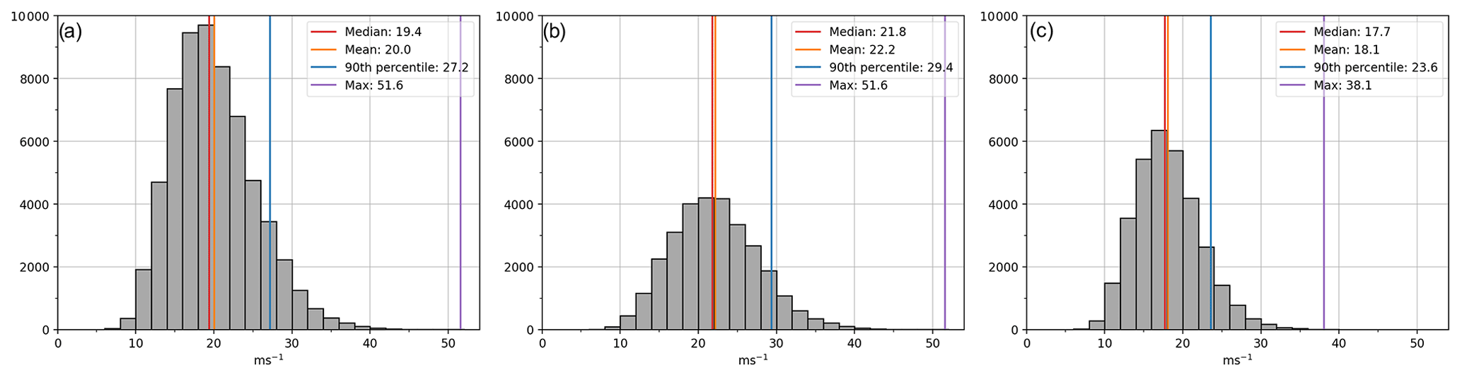
Figure 1Distribution of the maximum 10 m wind gust within 6∘ of the cyclone centre at each time step when the cyclone centre of the track is inside the northern Europe box during 1980–2019 covering (a) the whole year, (b) the cold season (October–March), and (c) the warm season (April–September).
In order to classify the extratropical cyclones based on their extremeness in wind gusts without depending on the season, we use 27.2 m s−1 (i.e. the 90th percentile of wind gusts during the whole year) as a threshold to divide the extratropical cyclones to windstorms and non-windstorms. The choice of 90th percentile as a threshold gives a reasonable number of windstorms for further analysis. When the windstorm threshold is equal in both seasons we can more easily compare the seasons since otherwise the warm-season windstorms would include extratropical cyclones that have lower wind gusts than cold-season windstorms. Furthermore, since our study focuses more on the dynamics and the structure of windstorms rather than impacts, the threshold we use considers wind gusts over the whole northern Europe box rather than only wind gusts over land. Therefore, our final cyclone classes are (1) all extratropical cyclones – all extratropical cyclones that have at least one track point inside the northern Europe box, (2) windstorms – extratropical cyclones whose associated wind gusts are equal to or exceed the 90th percentile when the cyclone centre is inside the northern Europe box, and (3) non-windstorms – extratropical cyclones whose associated wind gusts are below the 90th percentile when the cyclone centre is inside the northern Europe box. Hence, the sum of windstorms and non-windstorms equals all extratropical cyclones.
In this study, we also need to identify, for each windstorm, the time of the minimum MSLP and the time of the maximum 10 m wind gust. The time of the minimum MSLP is the time when the absolute minimum of MSLP occurs along the cyclone track, and therefore the cyclone centre does not need to be located within the northern Europe box at this time. In contrast, as we are interested in investigating wind gusts in northern Europe, we define the time of the maximum 10 m wind gust to be the time that the maximum gust occurs while the cyclone centre is within the northern Europe box. However, as the gusts are taken within a 6∘ radius of the cyclone centre, the location of the maximum gust can occur just outside of the northern Europe box. The locations of the minimum MSLP and the maximum 10 m wind gust for each windstorm track are shown in the Appendix Figs. A1 and A2.
3.3 Cyclone composites
To further examine the structure and evolution of northern Europe windstorms (identified as described in Sect. 3.2), we create cyclone composites in a similar way as for example Dacre et al. (2012) and Sinclair et al. (2020). The composites are produced for different meteorological variables at different offset times relative to two times: the time of the minimum MSLP and secondly the time of the maximum 10 m wind gust (these times are defined at the end of Sect. 3.2). For the compositing, the windstorms are transformed into a spherical grid (cyclone centre in the middle) and rotated to a cyclone-relative coordinate so that they all travel to the east. The composite for each meteorological variable and offset time is created by averaging that meteorological field of each individual windstorm.
3.4 Ensemble sensitivity analysis
To statistically identify precursors which are strongly correlated with characteristics of windstorms in northern Europe, we use an ensemble sensitivity analysis. In this study, “ensemble” refers to the population of extratropical cyclones that are defined as windstorms. The principle of the ensemble sensitivity method is to calculate the linear regression between a precursor field, x, and the so-called response function, J. In our study, we consider two response functions: (1) the minimum MSLP and (2) the maximum 10 m wind gust. The minimum MSLP was chosen because it is a common variable to represent the intensity of an extratropical cyclone, and the maximum wind gust was chosen because gusts usually cause the high impacts and damage. The minimum MSLP is not directly related to the wind gusts but indirectly by strengthening the pressure gradient, which is associated with stronger wind speeds and hence stronger wind gusts. The ensemble sensitivity analysis is applied to precursors on the cyclone centred radial grid.
The sensitivity S consists of multiplying three components:
where m is the linear regression slope, α is a correction factor, and σ is the standard deviation of the precursor. The linear regression slope m is calculated at each grid point (i,j):
The correlation factor α modifies the sensitivity S by giving less weight to slope values in those grid points that have weak correlations. This is done by defining α:
where ri,j is the correlation coefficient, and rmin is the threshold for correlations that are altered. Similarly to Dacre and Gray (2013), we set to be 0.05, which means that for all grid points where the correlation coefficient is less than 0.224, the sensitivity S is reduced.
The standard deviation σ is calculated at each grid point through all windstorms and over both seasons to ensure that the two seasons can be compared to each other. By multiplying with the standard deviation, the sensitivity S obtains the same units as the response function. Therefore, the sensitivity can be interpreted as how the response function (the minimum MSLP maximum 10 m wind gust) changes when there is an increase of 1 standard deviation in the precursor field.
The sign of the sensitivity is determined only by the regression slope m, and the magnitude is affected by all three components in Eq. (1). Negative sensitivity means that the precursor x and the response function J are negatively correlated. Regarding the response function of the minimum MSLP, this means that if the precursor increases it is associated with a decrease in the minimum MSLP, i.e. to a stronger windstorm in terms of MSLP. Likewise, regarding the response function of the maximum 10 m wind gust, negative sensitivity means that if the precursor increases it is associated with a decrease in the maximum wind gust. However, this implies that the windstorm gets weaker in terms of wind gusts. This is important to note when comparing the sensitivities of these response functions that the sign of the sensitivity indicates contrary evolution to the windstorm.
In our study, we examine four precursors: 850 hPa potential temperature anomaly, TCWV, 300 hPa wind speed, and 300 hPa PV. We selected these precursors because the 850 hPa potential temperature gradient is a main driver of extratropical cyclones through baroclinicity. TCWV allows us to investigate the availability of moisture that may influence diabatic processes, which further may affect the intensity of an extratropical cyclone. The 300 hPa wind speed describes the jet stream, and the location of an extratropical cyclone in relation to the jet stream is known to influence to the extratropical cyclone development. Lastly, the 300 hPa PV was chosen because the surface cyclone can intensify when it interacts with an upper-level trough, which can be interpreted from the upper-level PV field. The 850 hPa potential temperature is used as an anomaly to assess the strength of the temperature gradient. The anomaly is calculated in each individual windstorm separately by first area-averaging the 850 hPa potential temperature over the 18∘ radius composite and then subtracting this mean from each grid point in that windstorm. We investigate the precursor fields 24, 48, and 72 h before the time of the minimum MSLP or the maximum 10 m wind gust as defined in Sect. 3.2. These offset times are relevant because they occur at the typical range of extratropical cyclone predictability and evolution. In addition, since the ensemble sensitivity method uses linear correlations the sensitivities are most likely valid at short lead times, whereas at much longer lead times the non-linear affects would dominate.
The annual frequency of extratropical cyclones during 1980–2019 shows a large year-to-year variability in all three cyclone classes (Fig. 2). There are on average 149 extratropical cyclones every year that reach northern Europe (Fig. 2a), of which on average 35 cyclones, i.e. 23 %, are windstorms (Fig. 2c). Although the threshold for windstorms is the 90th percentile of wind gusts, the wind gust distribution can have multiple wind gust values per cyclone since we include all wind gust values at each time step when the cyclone centre is inside the northern Europe box. Hence, the ratio of windstorms can be higher than 10 %. The 40-year linear trends are not statistically significant in any of the three cyclone classes by using the Mann–Kendall test (Mann, 1945; Kendall, 1970) at the 5 % level. However, there is a decreasing trend (−3.7 cyclones per decade) in all extratropical cyclones (Fig. 2a and b) with a p value of 0.067, and therefore the trend would be significant with a 7 % level or higher. However, some time periods stand out with high or low annual number of extratropical cyclones. In the 1980s, there were overall more extratropical cyclones compared to the 40-year average (Fig. 2b), which was mainly due to the increased numbers of non-windstorms (Fig. 2f). In contrast, a longer-term drop in all extratropical cyclones (Fig. 2b) occurred between 1995–2005, during which time the number of windstorms (Fig. 2d) decreased more than the number of non-windstorms. The highest annual numbers of windstorms occurred in 1983 and 1990 (Fig. 2c and d).
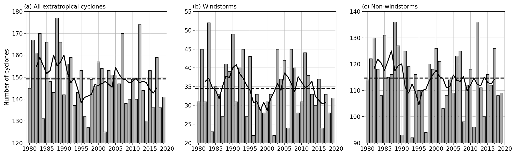
Figure 2Annual absolute numbers of extratropical cyclones in northern Europe in 1980–2019. Bars show the annual values, solid lines are 5-year running means, and dashed lines are annual means. (a) All extratropical cyclones, (b) windstorms, and (c) non-windstorms.
In addition to large inter-annual variability, we also investigated the seasonal cycle of the number of extratropical cyclones, windstorms, and non-windstorms (Fig. 3). Regarding all extratropical cyclones in northern Europe (Fig. 3a), the months from October to January and April have the highest median, between 13–15 extratropical cyclones per month, which means that on average almost every other day in these months an extratropical cyclone travels through northern Europe. The variability in extratropical cyclone numbers within each month (length of whiskers) is the highest during autumn and winter. Nevertheless, the monthly variation in the number of all extratropical cyclones does not have a significantly large seasonal cycle. In contrast, the number of windstorms (Fig. 3b) shows a strong annual cycle, with more windstorms in the cold season and less in the warm season. The highest median values of 5–6 windstorms per month are in January and December, whereas in May, June, and July, there are on average no windstorms at all. The variation in windstorm numbers within the cold-season months is, however, quite large; for example in November, the number of windstorms ranges from 0 to 14. The seasonal cycle for non-windstorms (Fig. 3c) is the opposite of that for windstorms with the highest number of non-windstorms occurring during the warm season from April to August. Therefore, we can conclude that while windstorms are more common in winter, and extratropical cyclones in summer are weaker, the overall number of extratropical cyclones per month in northern Europe does not differ considerably depending on season.

Figure 3Monthly distribution of cyclones in northern Europe. Orange lines are medians, boxes show first and third quartiles, and whiskers have a first value greater than and a last value less than IQR and IQR, respectively, where Q1 and Q3 are the first and third quartiles and IQR the interquartile range Q3–Q1. (a) All extratropical cyclones, (b) windstorms, and (c) non-windstorms.
The genesis and track densities are computed by the TRACK code using the spherical kernel method (Hodges, 1996), and the unit of the densities is number of cyclones per season (i.e. 6 months) per unit area, where the unit area is a 5∘ radius spherical cap (≈ 106 km2). In both seasons, the genesis region of all extratropical cyclones that affect northern Europe extends from the east coast of the United States to western Russia and from the Greenland Sea to the Mediterranean Sea (Fig. 4a and b). Most of the extratropical cyclones in the warm season originate over the land areas inside the northern Europe box (Fig. 4b). In the cold season (Fig. 4a), the most dense genesis region is broader, and, in addition to the land areas in northern Europe, most of the extratropical cyclones originate from the Norwegian Sea and the Barents Sea. The genesis over the east coast of the United States is more poleward in the warm season than in the cold season, which is in agreement with Priestley et al. (2020), who found that extratropical cyclones occur more equatorward in the winter than in the summer in the eastern North Atlantic.
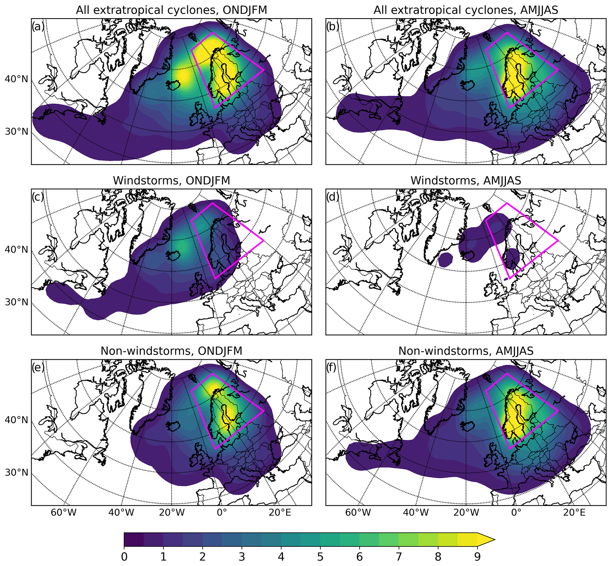
Figure 4Genesis density (number of cyclones per season (i.e. 6 months) per 5∘ spherical cap ≈ 106 km2) of (a, b) all extratropical cyclones, (c, d) windstorms, and (e, f) non-windstorms. The magenta box shows the northern Europe box where the tracks in this study are filtered to occur.
When considering windstorms and non-windstorms separately, there are distinct differences. Most of the non-windstorms originate over land areas in northern Europe (Fig. 4e and f), whereas windstorms have their genesis mostly over the Norwegian Sea and the Barents Sea (Fig. 4c and d). This also means that windstorms tend to originate farther away from northern Europe than non-windstorms. In addition, non-windstorms can originate over southern Europe while windstorms do not. In the cold season, the genesis region of windstorms is more zonally spread (Fig. 4c), whereas non-windstorms are more meridionally spread (Fig. 4e). In contrast, in the warm season the genesis region of non-windstorms is zonally spread and includes tracks from the eastern United States (Fig. 4f).
The track densities of all extratropical cyclones are, on a large scale, similar in both seasons, and the highest track density occurs inside the northern Europe box (Fig. 5a and b). Cold-season extratropical cyclones have high track densities over the eastern part of northern Europe and over the Barents Sea (Fig. 5a). There are somewhat fewer tracks over the Scandinavian Mountains, which is likely caused because the Scandinavian Mountains can, to some degree, modify the track of passing extratropical cyclones and even split the cyclone into two low centres (Grönås, 1997). When comparing windstorms and non-windstorms, it is evident that most windstorms have their cyclone centre at higher latitudes than non-windstorms (Fig. 5c–f). The difference is more pronounced in the cold season, when windstorms mostly occur over the Barents Sea (Fig. 5c), while non-windstorms occur over the southern parts of northern Europe (Fig. 5e).
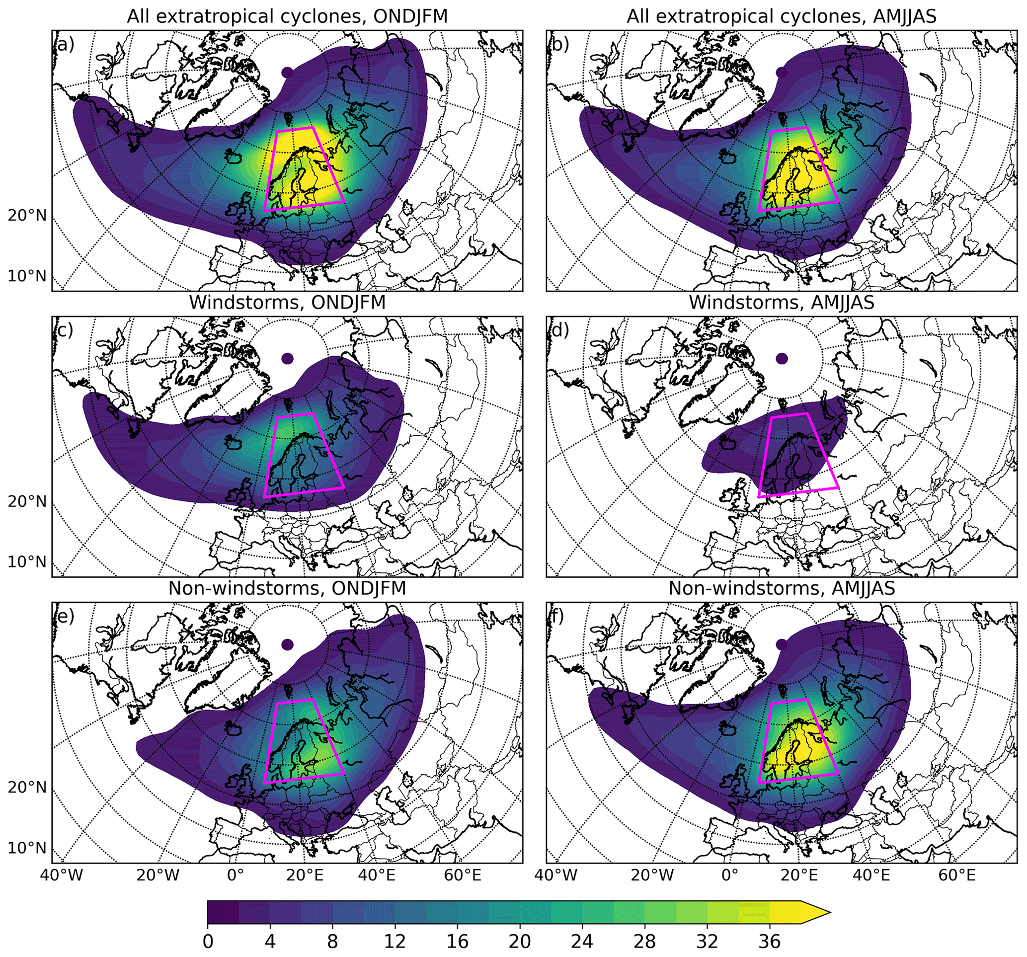
Figure 5Track density (number of cyclones per season (i.e. 6 months) per 5∘ spherical cap ≈ 106 km2) of (a, b) all extratropical cyclones, (c, d) windstorms, and (e, f) non-windstorms. The magenta box shows the northern Europe box where the tracks in this study are filtered to occur.
The majority of extratropical cyclones, regardless of the cyclone class (windstorm or non-windstorm) or season, propagate towards the east inside the northern Europe box (not shown). However, each year there is a small portion of extratropical cyclones that propagate towards the west, and this is slightly more visible in the warm season than in the cold season. This is also seen in the genesis density (Fig. 4), where some extratropical cyclones originate on the eastern edge of the northern Europe box.
The median duration of the cyclone lifetime with all extratropical cyclones is 3.4 d in the cold season and 3.6 d in the warm season (not shown). Considering windstorms, the median lifetime is 4 d in both the cold and warm seasons, while non-windstorms have a longer median lifetime in the warm season (3.6 d) than in the cold season (3 d, not shown). Therefore, extratropical cyclones in northern Europe are on average longer-lived in the warm season compared to the cold season and in windstorms compared to non-windstorms. The lifetime of extratropical cyclones, especially in the extremely long-lasting cases, can also be interpreted from the width of the histograms in Fig. 6. In the warm season the histogram is wider (from −13 to 17 d; Fig. 6b), indicating that the lifetimes are longer than in the cold season (from −9 to 10 d; Fig. 6a).
Figure 6 shows the maximum 10 m wind gusts in northern Europe (i.e. the maximum 10 m wind gust when the cyclone centre is inside the northern Europe box) in relation to the time of the minimum MSLP. The highest wind gust values on the y axis are concentrated close to zero on the x axis, which means that the maximum wind gusts occur close to the time of the minimum MSLP. The median occurrence time of the maximum gusts relative to the time of the minimum MSLP is 0 h for all extratropical cyclones and non-windstorms and +3 h for windstorms. There is no differences between the seasons on the median occurrence times. Overall, the occurrence time of the wind gusts is practically very close to the minimum MSLP, and the difference between windstorms and non-windstorms is small. In the cold season, the maximum 10 m wind gusts are higher (up to 52 m s−1) than in the warm season (up to 38 m s−1), which was also seen in the wind gust distributions (Fig. 1). Figure 6 also shows that while the wind gusts are the strongest at the time of the minimum MSLP, after that the wind gusts decrease. This happens especially in windstorms (Fig. 6c and d) where a negative tilt is visible after the time of the minimum MSLP. The negative tilt is not evident in non-windstorms (Fig. 6e and f), but non-windstorms by definition do not have strong wind gusts (there are no wind gust values above 27.2 m s−1).

Figure 6Normalized frequency of the maximum 10 m wind gust (m s−1) in northern Europe (i.e. the maximum 10 m wind gust when the cyclone centre is inside the northern Europe box) in relation to the time of the minimum mean sea level pressure (MSLP) during the cold season (a, c, e) and the warm season (b, d, f): (a, b) all extratropical cyclones, (c, d) windstorms, and (e, f) non-windstorms. Zero on the x axis indicates the time when the minimum MSLP during the track is obtained, and negative (positive) values indicate days before (after) that time. The frequency is normalized by the total number of the points in the tracks, and the colours are in a logarithmic scale. There are three data points with x-axis values over 12 d which are cut from the figure.
The composites of 10 m wind gust, MSLP and 850 hPa potential temperature are shown in Fig. 7 for the cold season and in Fig. 8 for the warm season, and these fields allow us to determine the spatial structure of windstorms in northern Europe. The offset times are relative to the time of the minimum MSLP of each windstorm (defined in Sect. 3.2). We investigate here the offset times at −48, −24, 0, and +24 h since Fig. 6 shows that these times cover the evolution before and after the strongest wind gusts and additionally include enough windstorms to ensure a reasonable number of cyclones in each composite; at the time of the minimum MSLP there are 1129 windstorms in the cold season and 245 windstorms in the warm season.
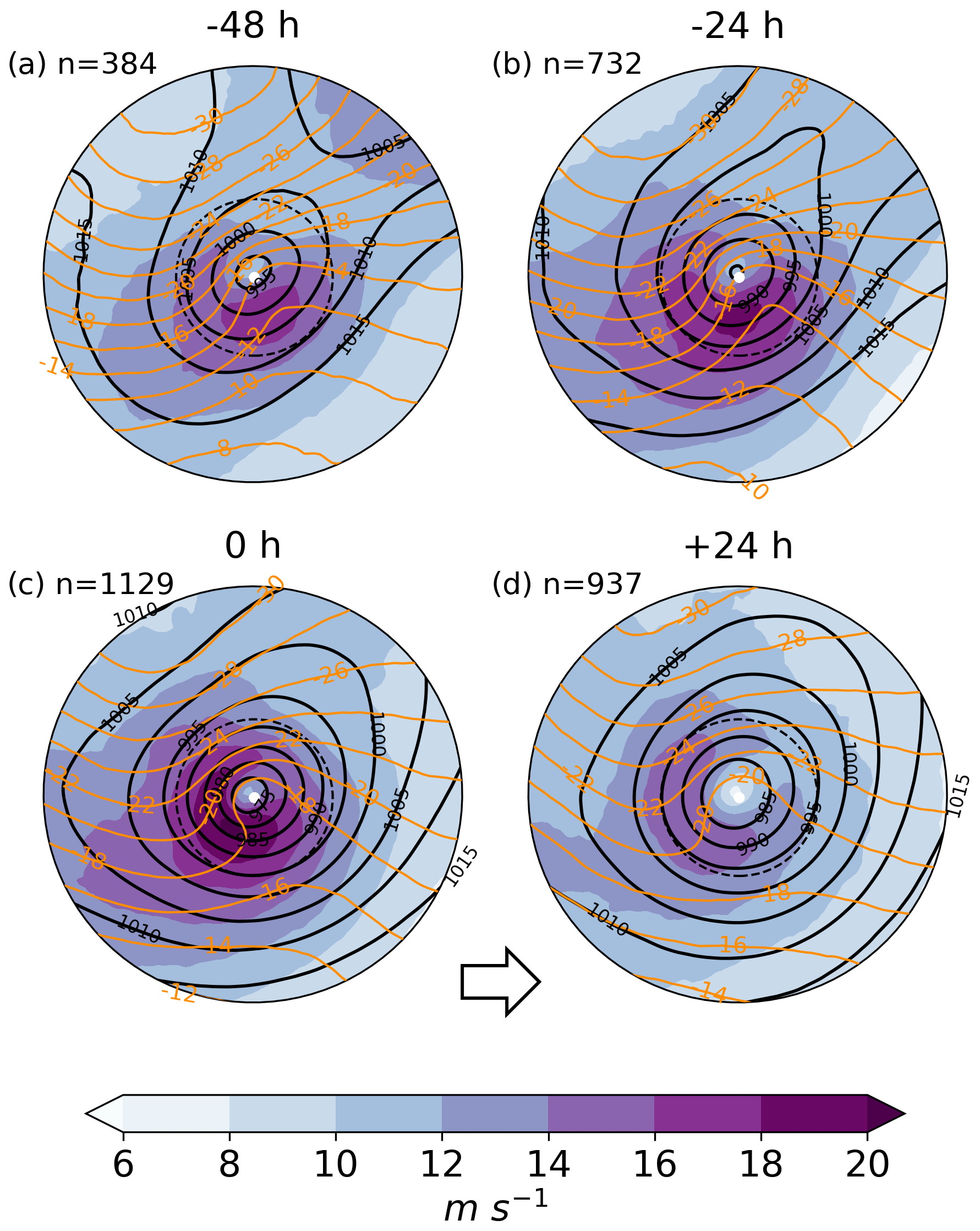
Figure 7The maximum 10 m wind gust (colours; m s−1), mean sea level pressure (black contours; 5 hPa interval), and 850 hPa potential temperature (orange contours; 2 ∘C interval) composites of windstorms during the cold season (October–March). The offset times are relative to the time of the minimum mean sea level pressure: (a) −48 h, (b) −24 (h, c) 0 h, and (d) +24 h. The number in each panel is the number of individual windstorms in each composite. The radius of the plots is 18∘, and the 6∘ radius is marked with a dashed circle. The arrow shows the propagation direction of the cyclones.
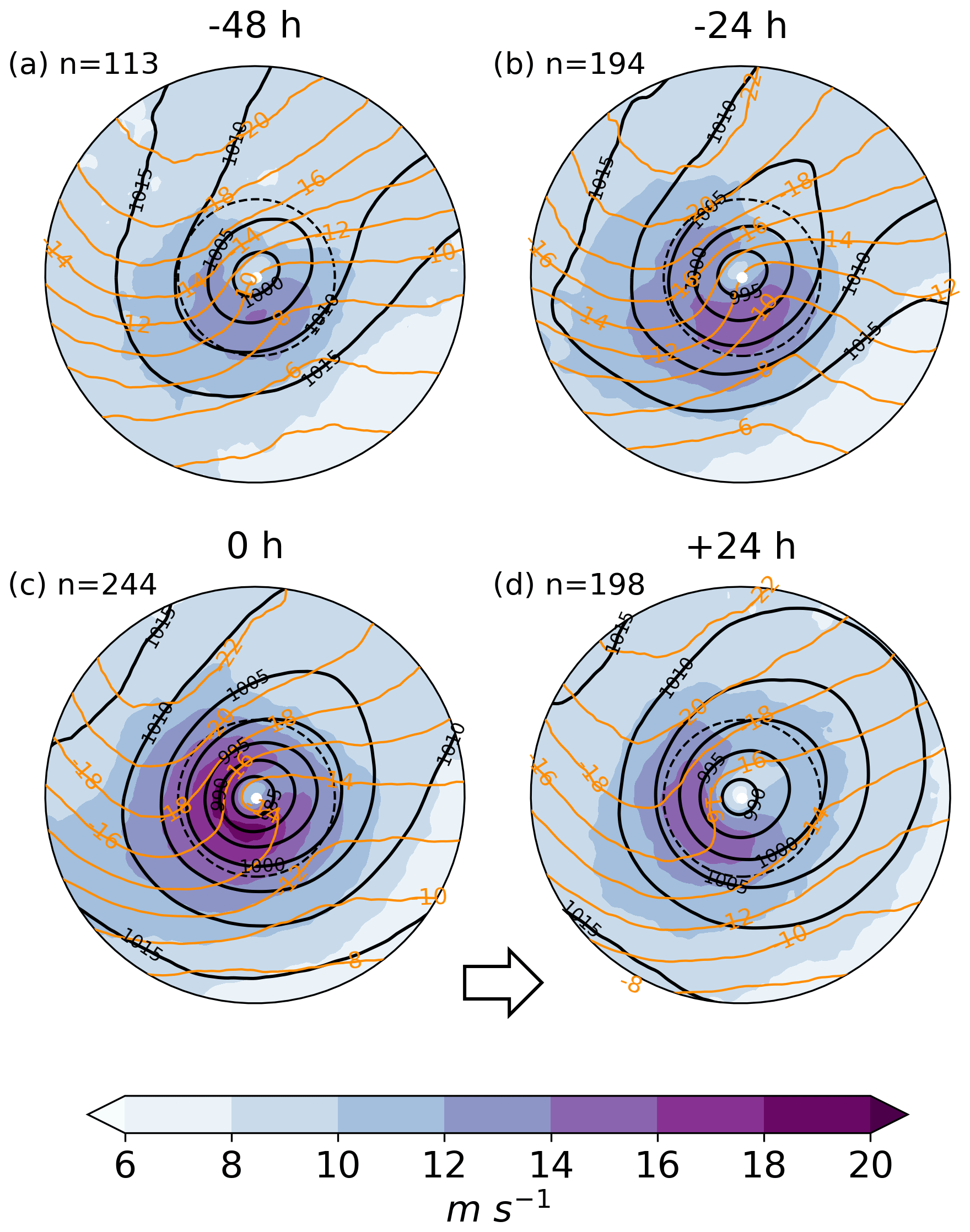
Figure 8The maximum 10 m wind gust (colours; m s−1), mean sea level pressure (black contours; 5 hPa interval), and 850 hPa potential temperature (orange contours; 2 ∘C interval) composites of windstorms during the warm season (April–September). The offset times are relative to the time of the minimum mean sea level pressure: (a) −48 h, (b) −24 h, (c) 0 h, and (d) +24 h. The number in each panel is the number of individual windstorms in each composite. The radius of the plots is 18∘, and the 6∘ radius is marked with a dashed circle. The arrow shows the propagation direction of the cyclones.
Already 48 h before the minimum MSLP (Figs. 7a and 8a), a closed low-pressure centre is evident in both seasons. The cold-season composite has a deeper central pressure (994 hPa) and a stronger pressure gradient than the warm-season composite (998 hPa). The frontal structure is visible from the 850 hPa potential temperature composite with a warm front downstream of the cyclone centre and a cold front upstream of the cyclone centre. The strongest wind gusts occur in the warm sector in the region of the strongest pressure gradient. In addition, the strongest wind gusts are located within a 6∘ radius from the cyclone centre, which supports the choice of selecting the maximum wind gust within 6∘. The strongest composite gusts are 17.2 m s−1 in the cold season and 14.2 m s−1 in the warm season. The region of the strongest gusts is more widely spread in the cold season than in the warm season. This indicates that the windstorms in the cold season are larger in spatial scale than in the warm season.
At 24 h before the minimum MSLP (Figs. 7b and 8b), the central pressure decreases, and the pressure and frontal gradients increase compared to the −48 h offset time. The wind gusts get stronger, while the maximum gust location spreads extending from the warm sector to the cold front. At the time of the minimum MSLP (Figs. 7c and 8c), the central pressure in the cold season is 972 hPa and in the warm season 981 hPa, and the pressure gradient is the strongest equatorward of the cyclone centre. The warm front starts to wrap around the cyclone centre, indicating that the windstorm is reaching its mature stage. The wind gusts are the strongest at this offset time, and the maximum gust values are 20.5 m s−1 in the cold season and 18.6 m s−1 in the warm season. The location of the maximum wind gusts occurs in a region extending from the warm sector to behind the cold front, where the pressure gradient is the strongest. The maximum wind gusts are still within a 6∘ radius from the cyclone centre. At 24 h after the minimum MSLP (Figs. 7d and 8d), the central pressure has risen and the frontal structure weakened. The maximum wind gusts have decreased and now occur behind the cold front.
To conclude, the location of the maximum wind gusts moves from the warm sector to behind the cold front following the location of the strongest pressure gradient during the evolution of the composite windstorm. The wind gusts, pressure gradient, and potential temperature gradient are all stronger and the minimum MSLP deeper in the cold season than in the warm season. In addition, the spatial scale of the windstorm is larger in the cold season than in the warm season.
In this section, we use the ensemble sensitivity analysis to investigate how two response functions, (1) the minimum MSLP and (2) the maximum 10 m wind gust, are sensitive to four different precursors at different offset times. The precursors we examine are 850 hPa potential temperature anomaly, TCWV, 300 hPa wind speed, and 300 hPa PV, and these are analysed 72, 48, and 24 h before the offset time.
7.1 Sensitivity of the minimum MSLP
The offset time in the minimum MSLP sensitivities is relative to the time when the minimum MSLP occurs during the whole lifetime of the windstorm (same as in the composites in Sect. 6). The 850 hPa potential temperature anomaly composites (contours in Fig. 9) show similar frontal structures and seasonal differences as in Figs. 7 and 8, which show the absolute values. In the cold season, the sensitivity to the 850 hPa potential temperature anomaly has a dipole pattern with negative sensitivity in the warm sector and positive sensitivity in the cold sector north of the cyclone centre. Negative sensitivity in the warm sector means that an increase in the 850 hPa potential temperature anomaly in this location is associated with a lower minimum MSLP. The strongest negative sensitivities at −48 h (Fig. 9c) show that an increase of 1 standard deviation in the 850 hPa potential temperature anomaly decreases the minimum MSLP by more than 13 hPa. Likewise, positive sensitivity in the cold sector means that an increase in the 850 hPa potential temperature anomaly in this location is associated with a higher minimum MSLP, which, in other words, means that a decrease in temperature in the cold sector is associated with a lower minimum MSLP. The strongest positive sensitivities at −72 h (Fig. 9a) and −48 h (Fig. 9c) show that an increase of 1 standard deviation in the 850 hPa potential temperature anomaly increases the minimum MSLP by 10 hPa. This implies that a stronger temperature gradient (i.e. a warmer warm sector and a colder cold sector) is associated with a deeper minimum MSLP and hence with a stronger windstorm in terms of MSLP. This is in agreement with studies that have shown that stronger baroclinicity and thus temperature gradient lead to a stronger extratropical cyclone (Tierney et al., 2018; Rantanen et al., 2019). The dipole pattern is evident in the cold season at all offset times, with the strongest sensitivities at −48 h. In the warm season, the dipole pattern is visible at −48 h (Fig. 9d) and −24 h (Fig. 9f) offset times, and the sensitivity at −48 h is distinctly higher than at −24 h. The minimum MSLP is not sensitive to the 850 hPa potential temperature anomaly at −72 h in the warm season (Fig. 9b).
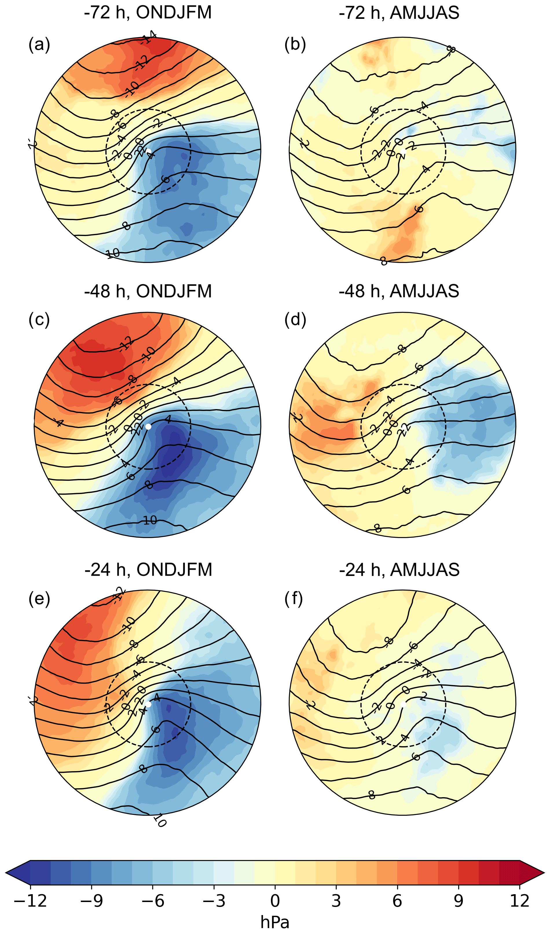
Figure 9Sensitivity of the minimum MSLP to the 850 hPa potential temperature anomaly (colours; hPa) and the composite mean of the 850 hPa potential temperature anomaly (contours; 2 ∘C interval) (a, b) 72 h, (c, d) 48 h, and (e, f) 24 h before the occurrence of the minimum MSLP. Note that the colour scale here is double that in the other sensitivity figures. The radius of the plots is 18∘, and the 6∘ radius is marked with a dashed circle.
The TCWV composites (contours in Fig. 10) have a similar pattern to the 850 hPa temperature anomaly composites, and the highest amount of moisture is found south of the cyclone centre in the warm sector. The negative sensitivities south and downstream of the cyclone centre mean that more moisture in the warm sector is associated with a deeper minimum MSLP. The sensitivities are higher in the cold season than in the warm season and have their largest values at −48 h offset time in both seasons. The highest sensitivity in the cold season is at −48 h offset time (Fig. 10c), where an increase of 1 standard deviation in TCWV decreases the minimum MSLP by 6 hPa. These results can be interpreted in a way that more moisture leads to more precipitation, and this leads to more diabatic heating. Furthermore, diabatic heating can then produce low-level positive PV, and this can further intensify the windstorm. Our result is consistent with Dacre et al. (2019), who similarly used ensemble sensitivity analysis to show that downstream moisture (TCWV) leads to an increase in total precipitation.

Figure 10Sensitivity of the minimum MSLP to the TCWV (colours; hPa) and the composite mean of TCWV (contours; 2 kg m−2 interval) (a, b) 72 h, (c, d) 48 h, and (e, f) 24 h before the occurrence of the minimum MSLP. The radius of the plots is 18∘, and the 6∘ radius is marked with a dashed circle.
The 300 hPa wind speed composites (contours in Fig. 11) show that the cyclone centre at −72 h is located in the centre of the poleward side of the jet stream, but at −48 and −24 h the cyclone centre is located at the left exit of the jet stream. The windstorm only starts strongly deepening at −48 h (not shown), when it moves into the left exit region (favourable region for cyclone development), and then 48 h later, at 0 h, the windstorm has its minimum MSLP. In the cold season at −72 h (Fig. 11a) and −48 h (Fig. 11c) offset times, the largest sensitivities are north-east of the cyclone centre. The strongest negative sensitivities in Fig. 11 mean that when the 300 hPa wind speeds increase by 1 standard deviation, it results in a decrease in minimum MSLP by 6 hPa. This implies that the minimum MSLP of a windstorm is deeper when the 300 hPa jet stream is extended north-east of the cyclone centre. A situation when the 300 hPa wind speed is stronger north-east of the cyclone centre suggests that the jet stream is tilted and thus more meridional. Furthermore, this implies that although at −72 h the cyclone centre is not located at the left exit of the jet, it possibly is in a region of cyclonic curvature vorticity advection. The 300 hPa wind speed at −24 h (Fig. 11e) has large sensitivities over the whole jet stream, meaning that the minimum MSLP decreases when the jet stream is stronger. In the warm season, there is more variability between the offset times than was observed in the cold season. The −24 h (Fig. 11f) sensitivity has a similar pattern to that of the cold season: a stronger jet stream is associated with a deeper windstorm. While the precursor at −48 h (Fig. 11d) shows some sensitivity for the north-east-extended jet stream, at −72 h (Fig. 11b) the field is more noisy and has no sensitivity. It is good to note that, climatologically, the jet stream is at a higher altitude in summer than in winter. However, the 300 hPa wind speed composites in the warm season do capture the jet streak, and the absolute 300 hPa wind speeds are not much weaker than in the cold season.
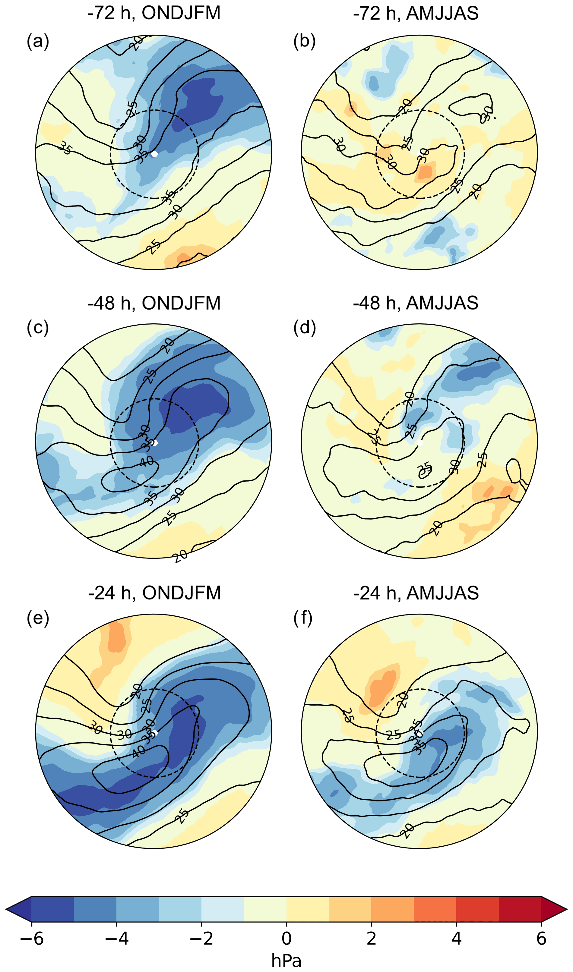
Figure 11Sensitivity of the minimum MSLP to the 300 hPa wind speed (colours; hPa) and the composite mean of 300 hPa wind speed (contours; 5 m s−1 interval) (a, b) 72 h, (c, d) 48 h, and (e, f) 24 h before the occurrence of the minimum MSLP. The radius of the plots is 18∘, and the 6∘ radius is marked with a dashed circle.
The 300 hPa PV composites (contours in Fig. 12) show high PV values (> 2 PVU, indicating stratospheric air) that occur upstream and north of the cyclone centre, denoting an upper-level trough. This westward tilt between a surface cyclone and an upper-level trough is typical in intensifying extratropical cyclones. An upper-level ridge (low PV values) is also seen downstream of the cyclone centre, with a PV gradient between the trough and the ridge, which corresponds to a tilted tropopause and thus the location of the jet stream. In the cold season, all offset times show that there is positive sensitivity in the warm sector, meaning that higher 300 hPa PV in that region is associated with an increase in the minimum MSLP. Quantitatively, an increase of 1 standard deviation in the 300 hPa PV is associated with an increase in the minimum MSLP by up to 5 hPa. In other words, lower PV in the warm sector is associated with a deeper windstorm. Lower PV in the warm sector implies a stronger upper-level ridge or higher tropopause, and this increases the PV gradient, i.e. steepens the tropopause. This is in agreement with the 300 hPa wind speed (Fig. 11): a steeper tropopause is consistent with a stronger jet stream. In addition to being sensitive to a stronger upper-level ridge, at −24 h (Fig. 12e) the minimum MSLP is also sensitive to a stronger upper-level trough, which similarly increases the PV gradient. In the warm season, the 300 hPa PV sensitivities are rather noisy and weak. This may imply that warm-season windstorms are less controlled by the upper-level vorticity advection and more by the low-level thermal advection or diabatic heating (more discussion on this in Sect. 8). Some sensitivity is visible to a stronger upper-level ridge at −48 h offset (Fig. 12d) and a stronger upper-level trough at −24 h offset (Fig. 12f), but mostly the minimum MSLP is not sensitive to the upper-level PV in warm-season windstorms.
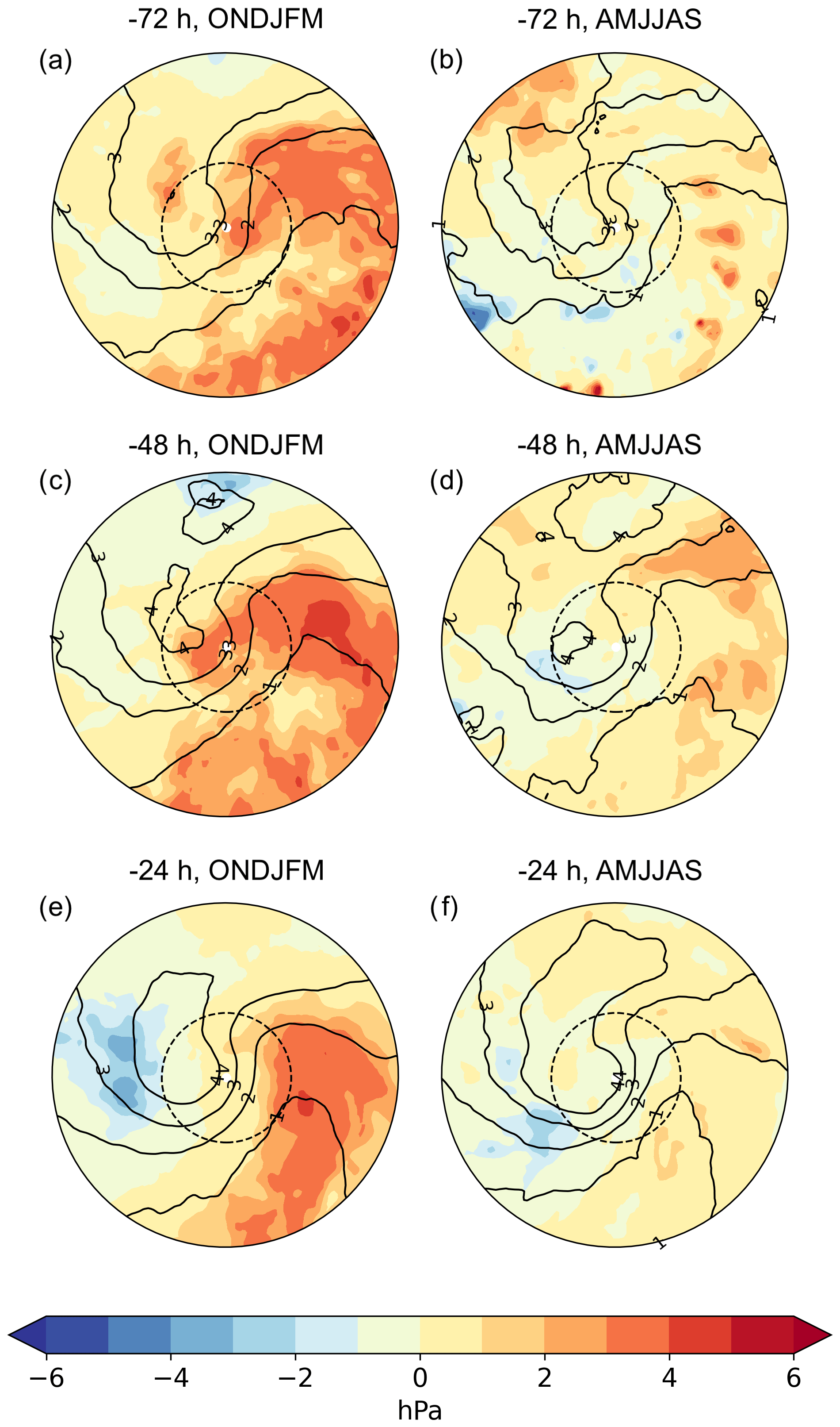
Figure 12Sensitivity of the minimum MSLP to the 300 hPa PV (colours; hPa) and the composite mean of 300 hPa PV (contours; 1 PVU interval, 1 PVU = m2 s−1 K kg−1) (a, b) 72 h, (c, d) 48 h, and (e, f) 24 h before the occurrence of the minimum MSLP. The radius of the plots is 18∘, and the 6∘ radius is marked with a dashed circle.
7.2 Sensitivity of the maximum 10 m wind gust
In the maximum 10 m wind gust sensitivities, the offset time is relative to the time when the maximum 10 m wind gust occurs when the cyclone centre is inside the northern Europe box. This means that the composite means are slightly different in this section compared to Sect. 7.1. The 850 hPa potential temperature anomaly composites (contours in Fig. 13) reveal that the frontal structure evolves within the 72 h before the maximum 10 m wind gust from a broad, large-scale temperature gradient with the beginnings of a frontal wave (Fig. 13a and b) to clearer frontal wave patterns (Fig. 13e and f). The sensitivity of the maximum 10 m wind gust has a similar dipole pattern to the sensitivity of the minimum MSLP, denoting that a stronger temperature gradient is associated with stronger gusts. This dipole pattern is visible in both seasons and all offset times. The strongest sensitivities are in the cold season and at −72 and −48 h offset times in two regions, in the warm sector and in the cold sector. An increase of 1 standard deviation in the 850 hPa potential temperature anomaly in the warm sector increases the maximum wind gust by 2.4 m s−1. An increase of 1 standard deviation in the 850 hPa potential temperature in the cold sector anomaly decreases the maximum wind gust by 2.0 m s−1.

Figure 13Sensitivity of the maximum 10 m wind gust to the 850 hPa potential temperature anomaly (colours; m s−1) and the composite mean of 850 hPa potential temperature anomaly (contours; 2 ∘C interval) (a, b) 72 h, (c, d) 48 h, and (e, f) 24 h before the occurrence of the maximum 10 m wind gust in northern Europe. The radius of the plots is 18∘, and the 6∘ radius is marked with a dashed circle.
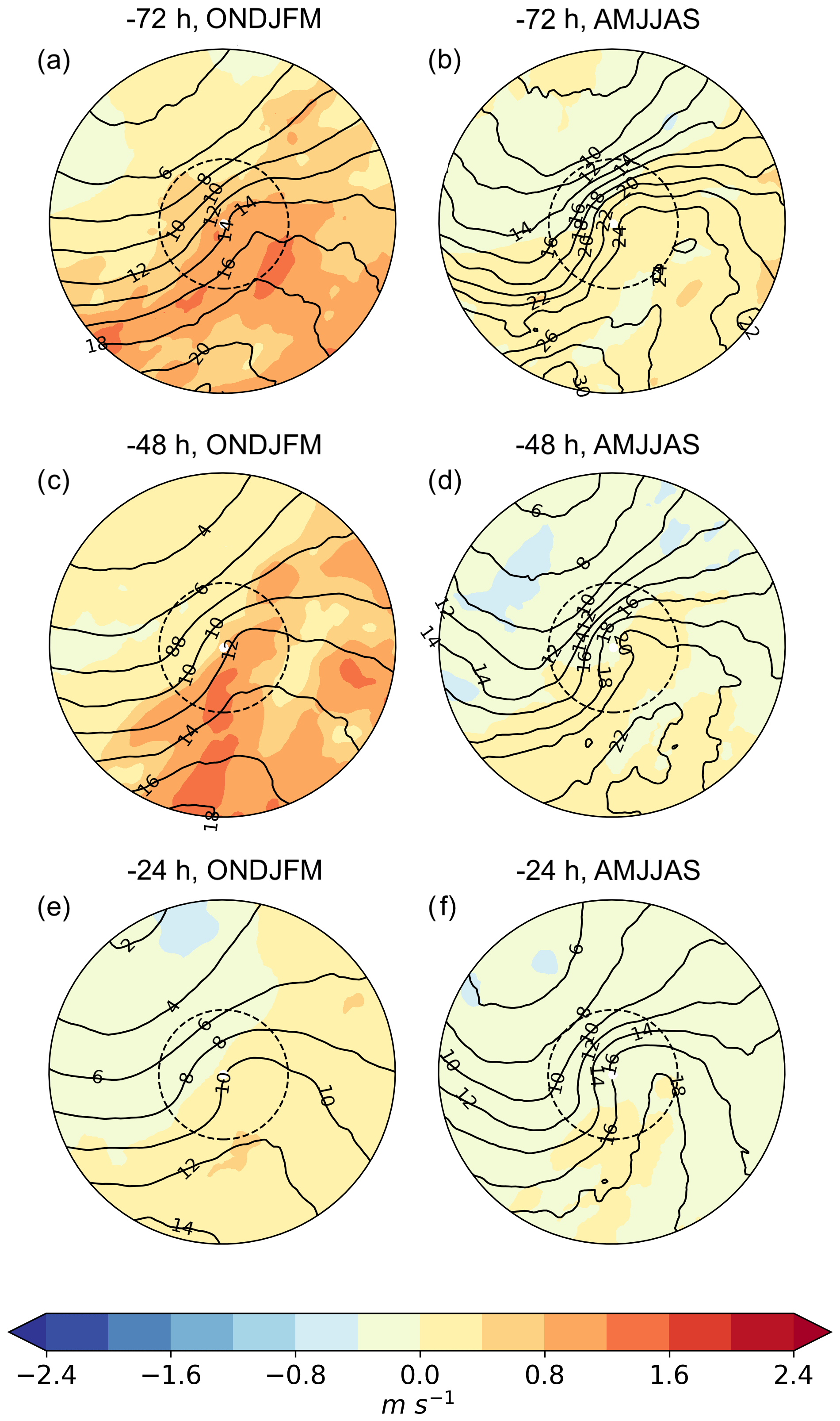
Figure 14Sensitivity of the maximum 10 m wind gust to the TCWV (colours; m s−1) and the composite mean of TCWV (contours; 2 kg m−2 interval) (a, b) 72 h, (c, d) 48 h, and (e, f) 24 h before the occurrence of the maximum 10 m wind gust in northern Europe. The radius of the plots is 18∘, and the 6∘ radius is marked with a dashed circle.
The TCWV composites (Fig. 14) are consistent with the frontal structure, with the highest TCWV values found in the warm sector. TCWV sensitivities show that in the cold season more moisture south of the cyclone centre 72 h (Fig. 14a) and 48 h (Fig. 14c) before the maximum 10 m wind gust occurrence is associated with stronger gusts. As discussed above, moisture may lead to diabatically produced low-level PV that deepens the minimum MSLP of the windstorm and hence increases the pressure gradient. The stronger pressure gradient then is associated with stronger wind gusts. The high sensitivities at −72 h are found in a broader area than at −48 h, where they are more concentrated near the cold front. The strongest sensitivities at −48 h offset (Fig. 14c) indicate that an increase of 1 standard deviation in TCWV in the warm sector increases the maximum wind gust by 1.6 m s−1. The TCWV sensitivities in the cold season at −24 h offset time and in the warm season at all offset times are weak, although the sensitivity patterns are similar.
The 300 hPa wind speed composites (contours in Fig. 15) show that in the cold season, the cyclone centre is located at the left exit region of the jet stream. The sensitivities in the cold season show that when the jet stream is farther north (and more downstream especially at −48 h), the wind gusts are stronger. An increase of 1 standard deviation in the 300 hPa wind speed north of the cyclone centre is associated with an increase in the maximum wind gusts by up to 1.6 m s−1. This suggests that stronger wind gusts occur in cold-season windstorms possibly when the jet stream is more poleward relative to the cyclone centre. The maximum wind gust is more sensitive to the jet stream at −72 h (Fig. 15a) and −48 h (Fig. 15c) offset times than −24 h (Fig. 15e) offset time. In the warm season, the cyclone centre is located at the centre of the poleward side of the jet stream. The warm-season sensitivities have a similar pattern to the cold season, but they are weaker: an increase of 1 standard deviation in the 300 hPa wind speed in the warm season is associated with an increase in the maximum wind gusts by up to 1.2 m s−1.
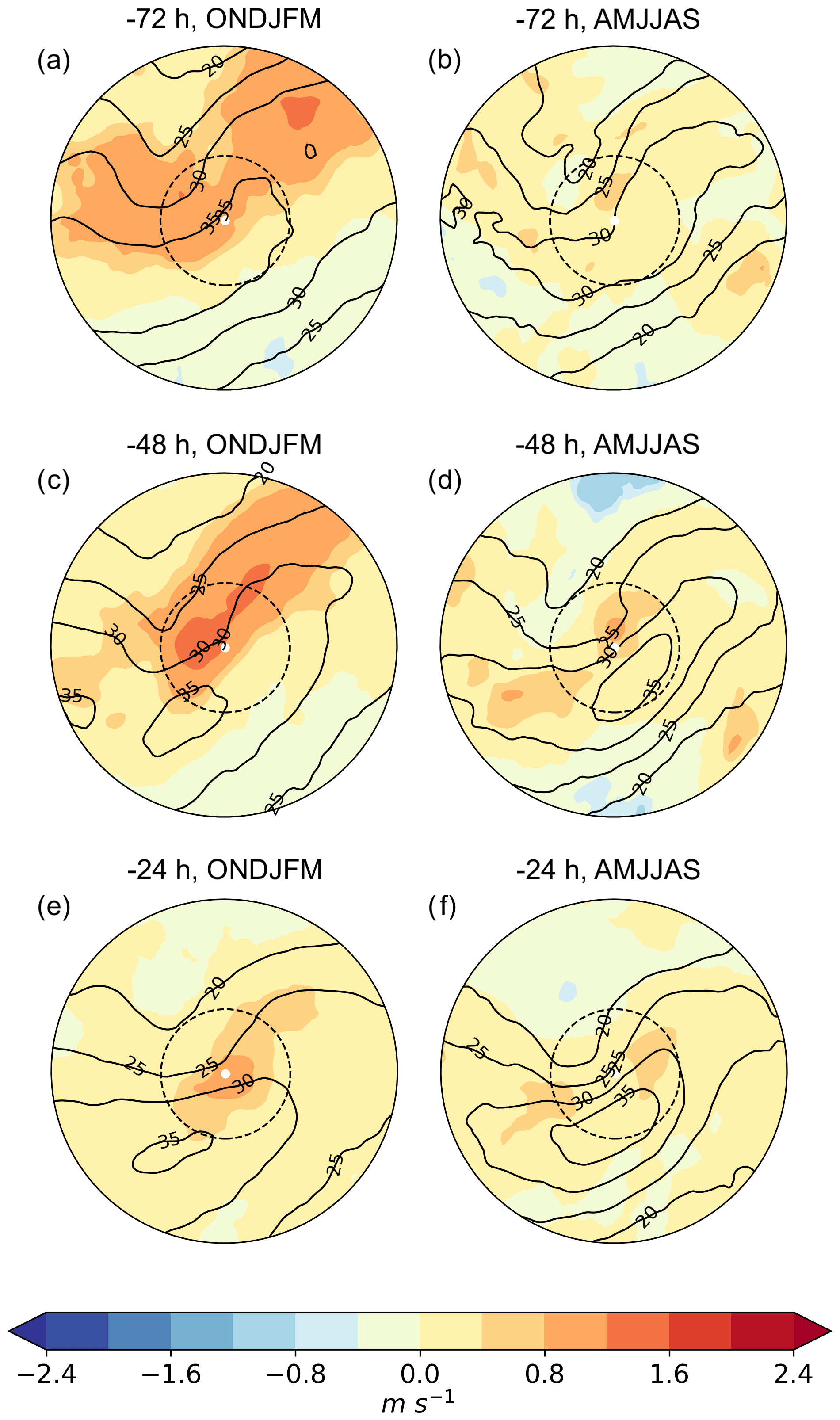
Figure 15Sensitivity of the maximum 10 m wind gust to the 300 hPa wind speed (colours; m s−1) and the composite mean of 300 hPa wind speed (contours; 5 m s−1 interval) (a, b) 72 h, (c, d) 48 h, and (e, f) 24 h before the occurrence of the maximum 10 m wind gust in northern Europe. The radius of the plots is 18∘, and the 6∘ radius is marked with a dashed circle.
Overall, the maximum 10 m wind gusts are weakly sensitive to the 300 hPa PV. In the cold season, −72 h (Fig. 16a) and −48 h (Fig. 16c) offset times show that a stronger upper-level ridge (i.e. lower PV values downstream of the cyclone centre) is associated with slightly stronger gusts. An increase of 1 standard deviation in the 300 hPa PV is associated with a decrease in the maximum wind gusts by 1.2 m s−1. This is not visible at −24 h or at any offset times in the warm season. However, in the warm season at −48 h offset time (Fig. 16d), there is weak sensitivity north and upstream of the cyclone centre, where an increase of 1 standard deviation in the 300 hPa PV (i.e. a stronger upper-level trough) is associated with an increase in the maximum wind gusts by 0.8 m s−1.
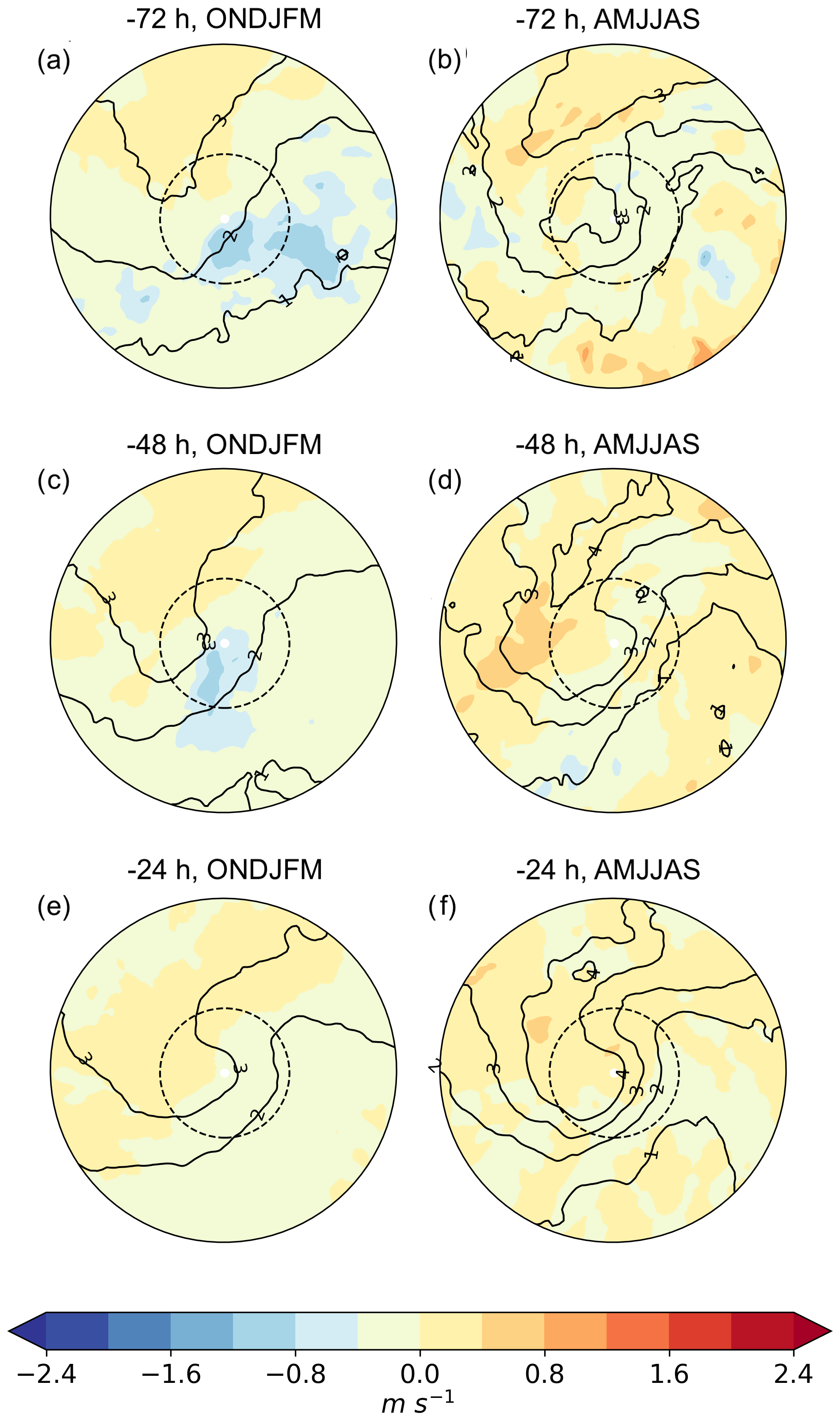
Figure 16Sensitivity of the maximum 10 m wind gust to the 300 hPa PV (colours; m s−1) and the composite mean of 300 hPa PV (contours; 1 PVU interval, 1 PVU = m2 s−1 K kg−1) (a, b) 72 h, (c, d) 48 h, and (e, f) 24 h before the occurrence of the maximum 10 m wind gust in northern Europe. The radius of the plots is 18∘, and the 6∘ radius is marked with a dashed circle.
This study investigated extratropical cyclones and windstorms in northern Europe and their characteristics, spatial and temporal evolution, and precursors. We tracked all extratropical cyclones in northern Europe during 1980–2019 and classified them into three classes: (1) all extratropical cyclones in northern Europe, (2) windstorms (i.e. extratropical cyclones which have strong wind gusts in northern Europe), and (3) non-windstorms (i.e. extratropical cyclones with no strong wind gusts in northern Europe). We investigated the cold season (October–March) and the warm season (April–September) separately to identify seasonal differences. We created cyclone composites to examine the cyclone evolution and used an ensemble sensitivity method to analyse precursors.
During the 40-year period, there is a large year-to-year variation in the annual number of extratropical cyclones, windstorms, and non-windstorms in northern Europe. The 40-year linear trends are not significant at the 95 % level; however, there is a decreasing trend in all extratropical cyclones (−3.7 cyclones per decade) that is significant at the 93 % level. Feser et al. (2015) reviewed the long-term trends of extratropical cyclone numbers over the North Atlantic and north-western Europe. They found that in their “Baltic Sea” region (covering the Baltic Sea; the Baltic states; and the major parts of Finland, Sweden, and Norway) there is no consensus on the long-term trends in reanalysis-, model- or, observation-based studies. Nonetheless, the sign and magnitude of linear trends depend strongly on the chosen time period and region, and therefore comparing different studies and results is difficult. In addition, it is important to note that a low number of windstorms in a specific year or decade does not mean that there could not be individual, strong windstorms. For example, our study shows that there were fewer windstorms than average between 1995–2005, while during this period a few extremely strong and damaging windstorms occurred in northern Europe: Storm Anatol in December 1999 (Ulbrich et al., 2001) and Storm Gudrun in January 2005 (Suursaar et al., 2006).
We found the well-known seasonality that windstorms are more common in winter, and extratropical cyclones in the warm season are weaker. However, a more unexpected result was that the overall number of extratropical cyclones per month in northern Europe does not differ much between months. This is contradictory to the general claim that there are less extratropical cyclones in the Northern Hemisphere during summer than winter (see for example the review by Ulbrich et al., 2009). However, this seasonal difference is most pronounced in the core of the North Atlantic storm track, while at the end of the storm track, i.e. in northern Europe, the difference is smaller (Hoskins and Hodges, 2019; Priestley et al., 2020). If considering the track densities in northern Europe, Hoskins and Hodges (2019) show mainly no difference between winter and summer, and Priestley et al. (2020) show only a small difference. Therefore, our finding does agree with other extratropical cyclone climatologies, but the other studies simply highlight more the general seasonality in the core of the storm track, although the seasonality has regional differences.
We investigated a set of cyclone characteristics to detect possible differences between windstorms and non-windstorms and between the cold and warm seasons. Windstorms tend to originate and occur over the sea areas (in the Norwegian and Barents seas), while non-windstorms originate and occur mostly over land in northern Europe. Partially, this is likely related to surface friction since we define windstorms based on their wind gusts, and winds are stronger over smooth surfaces, i.e. over sea areas. Moreover, the highest genesis densities of windstorms are co-located with the climatological left exit of the jet stream (Laurila et al., 2021), which is a favourable location for cyclone development. Our result also means that windstorms occur at higher latitudes than non-windstorms. This agrees with our composites, which showed that windstorms are located on the poleward side of the jet stream in both seasons. We additionally found that the maximum wind gusts occur approximately at the same time as the minimum MSLP regardless of the cyclone class or season.
The maximum wind gusts in windstorms move from the warm sector to behind the cold front during the cyclone evolution following the strongest pressure gradient. This shift in the maximum gust location during the cyclone evolution is in agreement with the shift in the maximum 900 hPa wind speeds of the 200 strongest extratropical cyclones in an aqua-planet study (Sinclair et al., 2020). In addition, the spatial patterns of MSLP and 850 hPa potential temperature in our composites are similar to the spatial patterns found by Catto et al. (2010) when they created composites of the 100 strongest extratropical cyclones in the Northern Hemisphere. This suggests that northern Europe windstorms have similar spatial and temporal structures to those found elsewhere in the Northern Hemisphere. Our results show that the wind gusts, pressure gradient, and temperature gradient are stronger, and the minimum MSLP is deeper in the cold season than in the warm season. The cold-season windstorms have their associated wind gusts covering a larger area and thus are spatially larger than warm-season windstorms. This is relevant when informing and preparing for likely impacts, yet it is important to note that our study only includes large-scale extratropical cyclones, whereas other weather systems (e.g. thunderstorms) can also cause strong winds and impacts.
Lastly, we investigated precursors to northern Europe windstorms for the minimum MSLP and the maximum 10 m wind gust. The first main conclusion of our precursor results is that cold-season windstorms have higher sensitivities and thus are potentially easier to forecast than warm-season windstorms in terms of both the minimum MSLP and the maximum wind gusts. Possible reasons for this are a higher case-to-case variability and more rare occurrence of warm-season windstorms compared to cold-season windstorms. The second main conclusion is that the minimum MSLP of a windstorm has higher sensitivities than its associated maximum wind gust. This is possibly caused by the different nature of these variables: MSLP is a larger-scale field, while wind gusts are more localized and turbulent. The third and last main conclusion is that the best precursor for northern Europe windstorms is the 850 hPa potential temperature anomaly, i.e. the temperature gradient. This precursor outperformed the TCWV (moisture), the 300 hPa wind speed (jet stream), and the 300 hPa PV (upper-level trough and tropopause steepness). This means that the 850 hPa temperature gradient has the strongest impact on the resulting minimum MSLP and the maximum wind gusts, and thus the temperature gradient is an important variable to follow when forecasting windstorms in northern Europe. If we apply our sensitivity results to climate change, the low-level temperature gradient is expected to decrease (IPCC, 2013), which based on our results would indicate weaker windstorms in terms of the minimum MSLP and the maximum wind gusts. However, this is counteracted by the atmospheric moisture, which is predicted to increase (IPCC, 2013) and hence would, based on our results from the TCWV sensitivities, indicate stronger windstorms.
The 300 hPa PV shows sensitivities to the downstream ridge, which is not found in Dacre and Gray (2013), who used the ensemble sensitivity analysis to investigate precursors to extratropical cyclones in the west and east North Atlantic. This difference between our and their results may be because of the difference in the geographical location: blocking is more common over northern Europe and Russia than over the North Atlantic (Pelly and Hoskins, 2003; Rimbu and Lohmann, 2011). The 300 hPa PV also gives weak or nonexistent sensitivities in the warm season. Petterssen and Smebye (1971) and Deveson et al. (2002) developed a cyclone development classification based on the upper- and lower-level forcing mechanisms, and they identified three types of cyclones. Type A cyclones develop due to lower-level thermal advection in baroclinic regions without a pre-existing upper-level trough; type B cyclones develop due to upper-level vorticity advection, where a pre-existing upper-level trough moves over an area of warm advection; and type C cyclones are characterized by strong latent heat release with initiation of strong upper-level forcing and weak low-level baroclinicity (Petterssen and Smebye, 1971; Deveson et al., 2002; Plant et al., 2003). Therefore, our result may indicate that warm-season windstorms in northern Europe are type A or type C cyclones since they are not dominated by upper-level forcing. Our finding that the TCWV gives weak sensitivities in the warm season was surprising since typically there is more diabatic heating in the warm season than in the cold season. However, this may be a result of a low number of windstorms and a high case-to-case variability in the warm season. Our results also showed that the sensitivities are generally higher at −48 h than at −24 h. One possible explanation could be that 24 h is too short of a time for the atmospheric available potential energy to be converted to kinetic energy, an energy conversion known as the Lorenz energy cycle (Lorenz, 1955).
Our study has certain limitations. There are multiple ways to classify extratropical cyclones and to define windstorms (Catto, 2016), and therefore, our results may depend on our windstorm definition. Due to different extratropical cyclone and windstorm definitions, direct comparison of our climatology to previous studies is not simple. We also made a subjective choice about what geographic area to study, and our results are likely to be sensitive to our choice of the box over northern Europe. The area we considered included sea areas, and most windstorms we identified occurred over sea, making our results less applicable to windstorms over land areas. Furthermore, our analysis was based solely on ERA5 reanalysis, which may not accurately capture wind gusts due to the coarse resolution of the reanalysis (∼31 km) and also because wind gusts are parameterized, not directly resolved. Another limitation is that composites (and climatological studies overall) smooth the case-to-case variability, and therefore there is still need for case studies to investigate different evolution paths in more detail. For example, Storm Aila occurred in Finland in September 2020 and developed in the right entrance of the jet stream (Rantanen et al., 2021), which is contradictory to our result that northern Europe windstorms occur poleward of the jet stream. On the other hand, Storm Aila formed in an area of a strong temperature gradient (Rantanen et al., 2021), which agrees with our results.
Despite the limitations noted above, our composite and sensitivity results highlight the common features of windstorms in northern Europe. This enhances our dynamical understanding of these potentially damaging weather systems and furthermore provides valuable guidance in the form of data-based “conceptual models” to weather forecasters in the region.
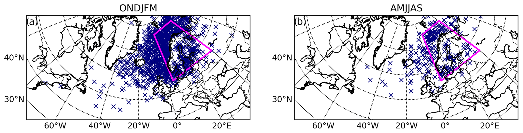
Figure A1The locations of the minimum MSLP of windstorm tracks. The time of the minimum MSLP is the time when the absolute minimum of MSLP occurs along the cyclone track.
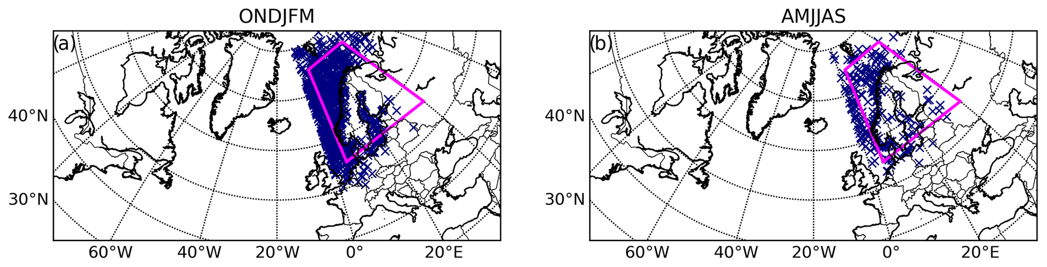
Figure A2The locations of the maximum 10 m wind gust of windstorm tracks. The time of the maximum 10 m wind gust is the time when the maximum wind gust occurs while the cyclone centre is within the northern Europe box.
Information on how to obtain the cyclone identification and tracking algorithm (TRACK) can be found from http://www.nerc-essc.ac.uk/~kih/TRACK/Track.html (last access: 18 November 2021, TRACK, 2021).
ERA5 reanalysis is available from the Copernicus Climate Change Service Climate Data Store (https://cds.climate.copernicus.eu/#!/search?text=ERA5&type=dataset, last access: 18 November 2021) (DOIs: https://doi.org/10.24381/cds.adbb2d47, https://doi.org/10.24381/cds.bd0915c6; Hersbach et al., 2018a, b).
TKL performed most of the data analysis, interpreted the results, drew the main conclusions, and wrote the majority of the paper. JC contributed to the data analysis of the wind speed distributions and the cyclone characteristics presented in Sects. 4, 5, and 6. VAS performed the cyclone tracking. VAS and HG conceived the study, provided guidance on the interpretation of the results, and led the overall scientific investigation. All authors provided comments on drafts of the manuscript.
The contact author has declared that neither they nor their co-authors have any competing interests.
Publisher’s note: Copernicus Publications remains neutral with regard to jurisdictional claims in published maps and institutional affiliations.
We thank Kevin Hodges for providing the cyclone tracking code TRACK and Helen Dacre for providing an initial version of the cyclone composite code. The authors wish to acknowledge CSC – IT Center for Science, Finland, for computational resources and ECMWF for providing the ERA5 reanalysis, which is available from the Copernicus Climate Change Service Climate Data Store. This work was supported by the MONITUHO project, the ERA4CS WINDSURFER project, and Academy of Finland Flagship funding (grant nos. 337549 and 337552).
This research has been supported by the Academy of Finland (grant nos. 337549 and 337552); the Maa- ja metsätalousministeriö (grant no. 647/03.02.06.00/2018); and the European Commission, Horizon 2020 Framework Programme (ERA4CS (grant no. 690462)).
This paper was edited by Silvio Davolio and reviewed by two anonymous referees.
Ancell, B. and Hakim, G. J.: Comparing adjoint-and ensemble-sensitivity analysis with applications to observation targeting, Mon. Weather Rev., 135, 4117–4134, 2007. a
Bjerknes, J.: On the structure of moving cyclones, Geofys. Publ., 1, 1–8, 1919. a
Bjerknes, J. and Solberg, H.: Life cycle of cyclones and the polar front theory of atmospheric circulation, Geofys. Publ., 3, 3–18, 1922. a
Blackmon, M. L.: A Climatological Spectral Study of the 500 mb Geopotential Height of the Northern Hemisphere, J. Atmos. Sci., 33, 1607–1623, https://doi.org/10.1175/1520-0469(1976)033<1607:ACSSOT>2.0.CO;2, 1976. a
Catto, J. L.: Extratropical cyclone classification and its use in climate studies, Rev. Geophys., 54, 486–520, https://doi.org/10.1002/2016RG000519, 2016. a
Catto, J. L., Shaffrey, L. C., and Hodges, K. I.: Can climate models capture the structure of extratropical cyclones?, J. Climate, 23, 1621–1635, 2010. a, b
Charney, J. G.: The dynamics of long waves in a baroclinic westerly current, J. Atmos. Sci., 4, 136–162, https://doi.org/10.1175/1520-0469(1947)004<0136:TDOLWI>2.0.CO;2, 1947. a
Dacre, H. F. and Gray, S. L.: Quantifying the climatological relationship between extratropical cyclone intensity and atmospheric precursors, Geophys. Res. Lett., 40, 2322–2327, https://doi.org/10.1002/grl.50105, 2013. a, b
Dacre, H., Hawcroft, M., Stringer, M., and Hodges, K.: An extratropical cyclone atlas: A tool for illustrating cyclone structure and evolution characteristics, B. Am. Meteorol. Soc., 93, 1497–1502, 2012. a, b, c
Dacre, H. F., Martinez-Alvarado, O., and Mbengue, C. O.: Linking atmospheric rivers and warm conveyor belt airflows, J. Hydrometeorol., 20, 1183–1196, 2019. a, b
Deveson, A. C. L., Browning, K. A., and Hewson, T. D.: A classification of FASTEX cyclones using a height-attributable quasi-geostrophic vertical-motion diagnostic, Q. J. Roy. Meteor. Soc., 128, 93–117, https://doi.org/10.1256/00359000260498806, 2002. a, b
Faranda, D., Messori, G., and Yiou, P.: Dynamical proxies of North Atlantic predictability and extremes, Scientific Reports, 7, 1–10, 2017. a
Feser, F., Barcikowska, M., Krueger, O., Schenk, F., Weisse, R., and Xia, L.: Storminess over the North Atlantic and northwestern Europe–A review, Q. J. Roy. Meteor. Soc., 141, 350–382, https://doi.org/10.1002/qj.2364, 2015. a
Field, P. R. and Wood, R.: Precipitation and cloud structure in midlatitude cyclones, J. Climate, 20, 233–254, 2007. a
Garcies, L. and Homar, V.: Ensemble sensitivities of the real atmosphere: application to Mediterranean intense cyclones, Tellus A, 61, 394–406, https://doi.org/10.1111/j.1600-0870.2009.00392.x, 2009. a
Gardiner, B., Schuck, A., Schelhaas, M.-J., Orazio, C., Blennow, K., and Bruce, N. (eds.): Living with storm damage to forests, What Science Can Tell Us 3, European Forest Institute, 2013. a
Grönås, S.: Mesoscale phenomena induced by mountains over Scandinavia and Spitsbergen, in: Workshop on Orography, 10–12 November 1997, 165–181 pp., ECMWF, available at: https://www.ecmwf.int/node/9656, last access: 18 November 2021, Shinfield Park, Reading, 1997. a
Hersbach, H., Bell, B., Berrisford, P., Biavati, G., Horányi, A., Muñoz Sabater, J., Nicolas, J., Peubey, C., Radu, R., Rozum, I., Schepers, D., Simmons, A., Soci, C., Dee, D., and Thépaut, J.-N.: ERA5 hourly data on single levels from 1979 to present, Copernicus Climate Change Service (C3S) Climate Data Store (CDS) [data set], https://doi.org/10.24381/cds.adbb2d47, 2018a. a
Hersbach, H., Bell, B., Berrisford, P., Biavati, G., Horányi, A., Muñoz Sabater, J., Nicolas, J., Peubey, C., Radu, R., Rozum, I., Schepers, D., Simmons, A., Soci, C., Dee, D., and Thépaut, J.-N.: ERA5 hourly data on pressure levels from 1979 to present, Copernicus Climate Change Service (C3S) Climate Data Store (CDS) [data set], https://doi.org/10.24381/cds.bd0915c6, 2018b. a
Hersbach, H., Bell, B., Berrisford, P., Hirahara, S., Horányi, A., Muñoz-Sabater, J., Nicolas, J., Peubey, C., Radu, R., Schepers, D., Simmons, A., Soci, C., Abdalla, S., Abellan, X., Balsamo, G., Bechtold, P., Biavati, G., Bidlot, J., Bonavita, M., De Chiara, G., Dahlgren, P., Dee, D., Diamantakis, M., Dragani, R., Flemming, J., Forbes, R., Fuentes, M., Geer, A., Haimberger, L., Healy, S., Hogan, R. J., Hólm, E., Janisková, M., Keeley, S., Laloyaux, P., Lopez, P., Lupu, C., Radnoti, G., de Rosnay, P., Rozum, I., Vamborg, F., Villaume, S., and Thépaut, J.-N.: The ERA5 Global Reanalysis, Q. J. Roy. Meteor. Soc., 146, 1999–2049, https://doi.org/10.1002/qj.3803, 2020. a
Hodges, K. I.: A General Method for Tracking Analysis and Its Application to Meteorological Data, Mon. Weather Rev., 122, 2573–2586, https://doi.org/10.1175/1520-0493(1994)122<2573:AGMFTA>2.0.CO;2, 1994. a, b
Hodges, K. I.: Feature Tracking on the Unit Sphere, Mon. Weather Rev., 123, 3458–3465, https://doi.org/10.1175/1520-0493(1995)123<3458:FTOTUS>2.0.CO;2, 1995. a
Hodges, K.: Spherical nonparametric estimators applied to the UGAMP model integration for AMIP, Mon. Weather Rev., 124, 2914–2932, 1996. a
Hodges, K. I.: Adaptive Constraints for Feature Tracking, Mon. Weather Rev., 127, 1362–1373, https://doi.org/10.1175/1520-0493(1999)127<1362:ACFFT>2.0.CO;2, 1999. a
Hodges, K. I., Lee, R. W., and Bengtsson, L.: A comparison of extratropical cyclones in recent reanalyses ERA-Interim, NASA MERRA, NCEP CFSR, and JRA-25, J. Climate, 24, 4888–4906, 2011. a, b
Holley, D. M.: The impacts of Storm Odette in eastern England, 24–26 September 2020, Weather, 76, 86–88, https://doi.org/10.1002/wea.3920, 2021. a
Hoskins, B. J. and Hodges, K. I.: New Perspectives on the Northern Hemisphere Winter Storm Tracks, J. Atmos. Sci., 59, 1041–1061, https://doi.org/10.1175/1520-0469(2002)059<1041:NPOTNH>2.0.CO;2, 2002. a, b, c, d, e
Hoskins, B. J. and Hodges, K. I.: The Annual Cycle of Northern Hemisphere Storm Tracks. Part I: Seasons, J. Climate, 32, 1743–1760, https://doi.org/10.1175/JCLI-D-17-0870.1, 2019. a, b
IPCC: Climate Change 2013: The Physical Science Basis. Contribution of Working Group I to the Fifth Assessment Report of the Intergovernmental Panel on Climate Change, Cambridge University Press, Cambridge, United Kingdom and New York, NY, USA, https://doi.org/10.1017/CBO9781107415324, 2013. a, b
Kendall, M. G.: Rank Correlation Methods, Griffin, London, ISBN 978-0-8526-4199-6, 1970. a
Krueger, O. and Von Storch, H.: Evaluation of an air pressure–based proxy for storm activity, J. Climate, 24, 2612–2619, 2011. a
Kufeoglu, S. and Lehtonen, M.: Cyclone Dagmar of 2011 and its impacts in Finland, in: IEEE PES Innovative Smart Grid Technologies, Europe, 1–6 pp., https://doi.org/10.1109/ISGTEurope.2014.7028868, 2014. a
Laurila, T. K., Sinclair, V. A., and Gregow, H.: Climatology, variability, and trends in near-surface wind speeds over the North Atlantic and Europe during 1979–2018 based on ERA5, Int. J. Climatol., 41, 2253–2278, https://doi.org/10.1002/joc.6957, 2021. a
Lorenz, E. N.: Available potential energy and the maintenance of the general circulation, Tellus, 7, 157–167, 1955. a
Mann, H. B.: Nonparametric tests against trend, Econometrica, 13, 245–259, https://doi.org/10.2307/1907187, 1945. a
Pelly, J. L. and Hoskins, B. J.: A new perspective on blocking, J. Atmos. Sci., 60, 743–755, 2003. a
Petterssen, S. and Smebye, S.: On the development of extratropical cyclones, Q. J. Roy. Meteor. Soc., 97, 457–482, 1971. a, b
Pinto, J. G., Spangehl, T., Ulbrich, U., and Speth, P.: Sensitivities of a cyclone detection and tracking algorithm: individual tracks and climatology, Meteorol. Z., 14, 823–838, 2005. a
Plant, R. S., Craig, G. C., and Gray, S. L.: On a threefold classification of extratropical cyclogenesis, Q. J. Roy. Meteor. Soc., 129, 2989–3012, https://doi.org/10.1256/qj.02.174, 2003. a
Priestley, M. D. K., Ackerley, D., Catto, J. L., Hodges, K. I., McDonald, R. E., and Lee, R. W.: An Overview of the Extratropical Storm Tracks in CMIP6 Historical Simulations, J. Climate, 33, 6315–6343, https://doi.org/10.1175/JCLI-D-19-0928.1, 2020. a, b, c, d, e, f
Rantanen, M., Räisänen, J., Sinclair, V. A., and Järvinen, H.: Sensitivity of idealised baroclinic waves to mean atmospheric temperature and meridional temperature gradient changes, Clim. Dyn., 52, 2703–2719, 2019. a
Rantanen, M., Laurila, T. K., Sinclair, V. A., and Gregow, H.: Storm Aila: An unusually strong autumn storm in Finland, Weather, 76, 306–312, https://doi.org/10.1002/wea.3943, 2021. a, b, c
Rimbu, N. and Lohmann, G.: Winter and summer blocking variability in the North Atlantic region – evidence from long-term observational and proxy data from southwestern Greenland, Clim. Past, 7, 543–555, https://doi.org/10.5194/cp-7-543-2011, 2011. a
Rudeva, I. and Gulev, S. K.: Composite analysis of North Atlantic extratropical cyclones in NCEP–NCAR reanalysis data, Mon. Weather Rev., 139, 1419–1446, 2011. a
Schultz, D. M., Keyser, D., and Bosart, L. F.: The effect of large-scale flow on low-level frontal structure and evolution in midlatitude cyclones, Mon. Weather Rev., 126, 1767–1791, 1998. a
Shapiro, M. A. and Keyser, D.: Fronts, jet streams and the tropopause, in: Extratropical Cyclones: The Erik Palmén Memorial Volume, edited by: Newton, C. and Holopainen, E. O., American Meteorological Society, Boston, MA, 167–191, Online ISBN 978-1-944970-33-8, 1990. a
Sinclair, V. A., Rantanen, M., Haapanala, P., Räisänen, J., and Järvinen, H.: The characteristics and structure of extra-tropical cyclones in a warmer climate, Weather Clim. Dynam., 1, 1–25, https://doi.org/10.5194/wcd-1-1-2020, 2020. a, b, c
Suursaar, U., Kullas, T., Otsmann, M., Saaremae, I., Kuik, J., and Merilain, M.: Cyclone Gudrun in January 2005 and modelling its hydrodynamic consequences in the Estonian coastal waters, Boreal Environ. Res., 11, 143–159, 2006. a, b
Tervo, R., Láng, I., Jung, A., and Mäkelä, A.: Predicting power outages caused by extratropical storms, Nat. Hazards Earth Syst. Sci., 21, 607–627, https://doi.org/10.5194/nhess-21-607-2021, 2021. a
Tierney, G., Posselt, D. J., and Booth, J. F.: An examination of extratropical cyclone response to changes in baroclinicity and temperature in an idealized environment, Clim. Dynam., 51, 3829–3846, 2018. a
TRACK: Homepage, available at: http://www.nerc-essc.ac.uk/~kih/TRACK/Track.html, last access: 18 November 2021. a
Ulbrich, U., Fink, A., Klawa, M., and Pinto, J. G.: Three extreme storms over Europe in December 1999, Weather, 56, 70–80, 2001. a
Ulbrich, U., Leckebusch, G., and Pinto, J. G.: Extra-tropical cyclones in the present and future climate: a review, Theor. Appl. Climatol., 96, 117–131, 2009. a, b
Wang, C.-C. and Rogers, J. C.: A composite study of explosive cyclogenesis in different sectors of the North Atlantic. Part I: Cyclone structure and evolution, Mon. Weather Rev., 129, 1481–1499, 2001. a, b
- Abstract
- Introduction
- ERA5 reanalysis data
- Methods
- Annual and monthly frequencies of extratropical cyclones, windstorms, and non-windstorms
- Characteristics of extratropical cyclones, windstorms, and non-windstorms
- Spatial and temporal evolution of maximum wind gusts, MSLP, and frontal structure in windstorms
- Precursors to windstorms
- Discussion and conclusions
- Appendix A
- Code availability
- Data availability
- Author contributions
- Competing interests
- Disclaimer
- Acknowledgements
- Financial support
- Review statement
- References