Storm track response to uniform global warming downstream of an idealized sea surface temperature front

The future evolution of storm tracks, their intensity, shape, and location, is an important driver of regional precipitation changes, cyclone-associated weather extremes, and regional climate patterns. For the North Atlantic storm track, Coupled Model Intercomparison Project (CMIP) data indicate a tripole pattern of change under the RCP8.5 scenario. In this study, the tripole pattern is qualitatively reproduced by simulating the change of a storm track generated downstream of an idealized sea surface temperature (SST) front under uniform warming on an aquaplanet. The simulated tripole pattern consists of reduced eddy kinetic energy (EKE) upstream and equatorward of the SST front, extended and poleward shifted enhanced EKE downstream of the SST front, and a regionally reduced EKE increase at polar latitudes. In the absence of the idealized SST front, in contrast, the storm track exhibits a poleward shift but no tripole pattern. A detailed analysis of the EKE and eddy available potential energy (EAPE) sources and sinks reveals that the changes are locally driven by changes in baroclinic conversion rather than diabatic processes. However, globally the change in baroclinic conversion averages to zero; thus the observed global EAPE increase results from diabatic generation. In particular, resolved-scale condensation plus parameterized cloud physics dominate the global EAPE increase followed by longwave radiation. Amplified stationary waves affect EKE and EAPE advection, which contributes to the local EKE and EAPE minimum at polar latitudes. Feature-based tracking provides further insight into cyclone life cycle changes downstream of the SST front. Moderately deepening cyclones deepen less in a warmer climate, while strongly deepening cyclones deepen more. Similarly, the average cyclone becomes less intense in a warmer climate, while the extremely intense cyclones become more intense. Both results hold true for cyclones with genesis in the vicinity of the SST front and elsewhere. The mean cyclone lifetime decreases, while it increases for those cyclones downstream of the SST front. The mean poleward displacement between genesis and maximum intensity increases for the most intense cyclones, while averaged over all cyclones there is a mild reduction and the result depends on the definition of the displacement. Finally, the number of cyclones decreases by approximately 15 %. Aquaplanet simulations with a localized SST front thus provide an enriched picture of storm track dynamics and associated changes with warming.

1 Introduction

The variability of storm tracks is of paramount importance in understanding regional climate patterns and their change (Shepherd, 2014). A complete mechanistic understanding of projected future storm track changes is still lacking because main factors underlying the variability of storm tracks compete with each other (Shaw et al., 2016; Shaw, 2019). Scientific attention has thus shifted to the analysis of these forcing factors across model hierarchies and to studies that attempt to isolate the importance of individual factors for future storm track activity.

Individual factors contributing to projected storm track changes have received enhanced consideration in recent years, in particular lower- and upper-level baroclinicity and increased diabatic processes. Enhanced upper-level baroclinicity, which results from lower-stratospheric cooling and tropical warming, is found to make waves with low wavenumbers more unstable and short wavenumbers more stable with the former being more capable of pushing the jet poleward (Rivière, 2011). Thus, a poleward shift and a change in the eddy length scale is observed under warming (Kidston et al., 2010; Rivière, 2011). This was recently confirmed by Chemke and Ming (2020), noting that large-scale waves will be stronger at the end of the century, while the opposite was found for small-scale waves. However, an increase in humidity favors the development of more cyclonically breaking waves, which thus may – at least partly – counteract the previous mechanism as these waves push the jet equatorward (Orlanski, 2003). Further, there is good reason to assume that the tropical widening in response to global warming, which is a robust feature in climate models (Lu et al., 2007; Hu et al., 2013), adds to the poleward displacement of the midlatitude storm tracks (Kushner et al., 2001; Yin, 2005; Simpson et al., 2014). Indeed, increased dry static stability in the tropics is able to shift the storm tracks poleward, which may or may not occur in tandem with a widening of the Hadley cell (Mbengue and Schneider, 2013). Similar holds true for increased subtropical stability on the equatorward side of the jet in general (Lu et al., 2007, 2010). More recently, the enhanced poleward propagation of extratropical cyclones has been pinpointed as another crucial factor for the poleward shift of the storm tracks (Tamarin-Brodsky and Kaspi, 2017). This is motivated by the fact that increased deepening rates are inherently connected to enhanced poleward motion (Gilet et al., 2009; Coronel et al., 2015; Tamarin and Kaspi, 2016; Besson et al., 2021). Consequently, simulations with idealized warming or positive sea surface temperature (SST) anomalies, which are both key ingredients known to intensify cyclone deepening rates, all display an enhanced poleward deflection and shift of the storm tracks, at least for the very intense storms (Palmer and Zhaobo, 1985; Brayshaw et al., 2008; Kodama and Iwasaki, 2009; Graff and LaCasce, 2012; Tamarin and Kaspi, 2017).

The two main storm tracks in the Northern Hemisphere are located over the North Atlantic and North Pacific oceans and downstream of the western boundary currents, i.e., the Gulf Stream and Kuroshio Extension. The western boundary currents amplify the land–sea contrast and contribute to the anchoring of the oceanic storm tracks as they help maintain a near-surface zone of enhanced baroclinicity and supply heat and moisture from below by means of sensible and latent heat fluxes (Chang et al., 2002; Kelly et al., 2010; Sampe et al., 2010; Deremble et al., 2012; Booth et al., 2012a; Brayshaw et al., 2011; Papritz and Spengler, 2015). The SST fronts locally reinforce the meridional temperature gradient by warming via sensible heat flux where it is warmer and cooling where it is colder (Hotta and Nakamura, 2011). These reinforcements occur mainly between rather than during the passage of cyclones and fronts (Marcheggiani and Ambaum, 2020; Reeder et al., 2021; Tsopouridis et al., 2021). Thus, the SST front acts to pre-condition the environment for subsequent cyclones. Globally, the meridional temperature gradient is maintained by the differential solar irradiance. Locally, the combination of enhanced moisture storage capacity in a warmer climate and latent heat supply from below makes SST fronts prone to explosive moist cyclogenesis; in particular the downstream sector is of interest because condensation in extratropical cyclones occurs later during the life cycle. However, there is evidence that diabatic heating within storms tends to amplify their growth rates (e.g., Kuo et al., 1991; Davis et al., 1993; Stoelinga, 1996; Chang et al., 2002; Schemm et al., 2013). At the same time, transient diabatic processes, including surface fluxes, have been found to reduce eddy available potential energy (EAPE) and, thus, the reservoir from which eddy kinetic energy (EKE) can be generated (Ulbrich and Speth, 1991; Chang and Zurita-Gotor, 2007; Marcheggiani and Ambaum, 2020). This might occur, for example, if diabatic heating occurs on the poleward side of the jet and thereby reduce baroclinicity (i.e., the mean available potential energy) (Laîné et al., 2011). This influence of the transient diabatic heating by moist processes must not be confused with the diabatic influence of the hemispheric-wide radiation that makes a positive contribution to the mean available potential energy (Oort, 1964; Oort and Peixóto, 1974). Hence, on the scale of individual storms, increased diabatic heating in a warmer climate must also occur “in the right location” to help with the deepening (Kirshbaum et al., 2018). Further, individual storms must optimize their vertical tilt magnitude and tilt orientation to maximize their baroclinic growth efficiency (Davies and Bishop, 1994; Schemm and Rivière, 2019). The baroclinic conversion efficiency relates to the eddy diffusivity of storm tracks (Eq. 9 in Schemm and Rivière, 2019), which is a key quantity that controls the amplitude and transport characteristics of baroclinic eddies (Held and Larichev, 1996; Lapeyre and Held, 2003; Schemm and Schneider, 2018). Its response to warming is largely unknown, but changes in the vertical structure of storms have been reported by earlier idealized studies (Booth et al., 2012b; Tierney et al., 2018; Kirshbaum et al., 2018; Sinclair et al., 2020) suggesting that the baroclinic conversion efficiency and thus the storm-track diffusivity might change under warming (Caballero and Hanley, 2012).

The storm track response downstream of western boundary currents is complex and might differ from the storm track response seen in zonally uniform idealized warming experiments. The extent to which the storm tracks that form downstream of a major SST front react differently than others remains open, though some studies already give an indication. For example, Brayshaw et al. (2008) and Graff and LaCasce (2012) showed that an increase in the SST gradient in the extratropics increases the strength of the storm tracks but only if the SST gradients increase not too close to the subtropical jet. Uniform idealized global warming experiments, which do not change the SST gradients, have yielded mixed results. In the studies of Graff and LaCasce (2012) and Sinclair et al. (2020), the storm tracks appear to shift poleward, and strengthen and extend vertically. In Kodama and Iwasaki (2009) the jet and the storm track also shift poleward and the upper-level meridional temperature gradient increases due to enhanced tropical heating (in agreement with Sinclair et al., 2020), but the global mean eddy activity does not change in Kodama and Iwasaki (2009).

Main research questions

In this study, a localized SST gradient is added to a zonally uniform SST distribution to mimic a western boundary current and to create a regional storm track. This study aims to establish the archetypal response of a storm track generated downstream of a SST front to uniform global warming. The experiment is motivated by the fact that the two main storm tracks in the Northern Hemisphere originate downstream of western boundary currents. The reduced complexity of an aquaplanet appears attractive to provide a clearer picture of the partially opposing process-level changes found in studies based on CMIP data. Future studies will explore the sensitivity of the result to the SST front gradient, strength, and position, but here the focus is on the response to simple uniform warming. The response is described in terms of changes of the eddy energy cycle, that is EAPE and EKE, and the associated tendencies, including baroclinic, barotropic, and diabatic conversions, as well as the baroclinic conversion efficiency. The eddy energy cycle is widely used and allows for a comparison with existing studies. We also discuss the stationary wave and jet response to warming, but our focus is on the EKE and EAPE sources and sinks. Further, we analyze basic aspects from a feature-based perspective, such as changes in the lifetime, deepening rates, and poleward displacement. We systematically compare cyclones that develop downstream of the SST front to all other cyclones, in particular to those in the opposite hemisphere, for which we do not prescribe a SST front.

2 Simulation design and diagnostics

2.1 Idealized aquaplanet simulations with SST front

This study uses the Icosahedral Nonhydrostatic Weather and Climate Model (ICON; Zängl et al., 2015) initially developed in a joint collaboration between the German Weather Service (DWD) and the Max Planck Institute for Meteorology (MPI-M) and also in pre-operational use at the Swiss National Weather Service (MeteoSwiss). The model runs on an icosahedral grid with an effective horizontal resolution of approximately 80 km (called R02B05 in the ICON framework). It has 70 levels in the vertical, and the model top is placed at 65 km. The model employs a set of standard sub-grid-scale parameterizations used for numerical weather prediction purposes. These include in particular a one-moment two-category microphysics scheme (Doms et al., 2011), a convection scheme following Tiedtke (1989), a prognostic turbulent kinetic energy (TKE) scheme for sub-grid-scale turbulent transfer (Doms et al., 2011), and a parameterization for non-orographic gravity wave drag (Orr et al., 2010). For radiation, the ecRad scheme is used (Hogand and Bozzo, 2018).

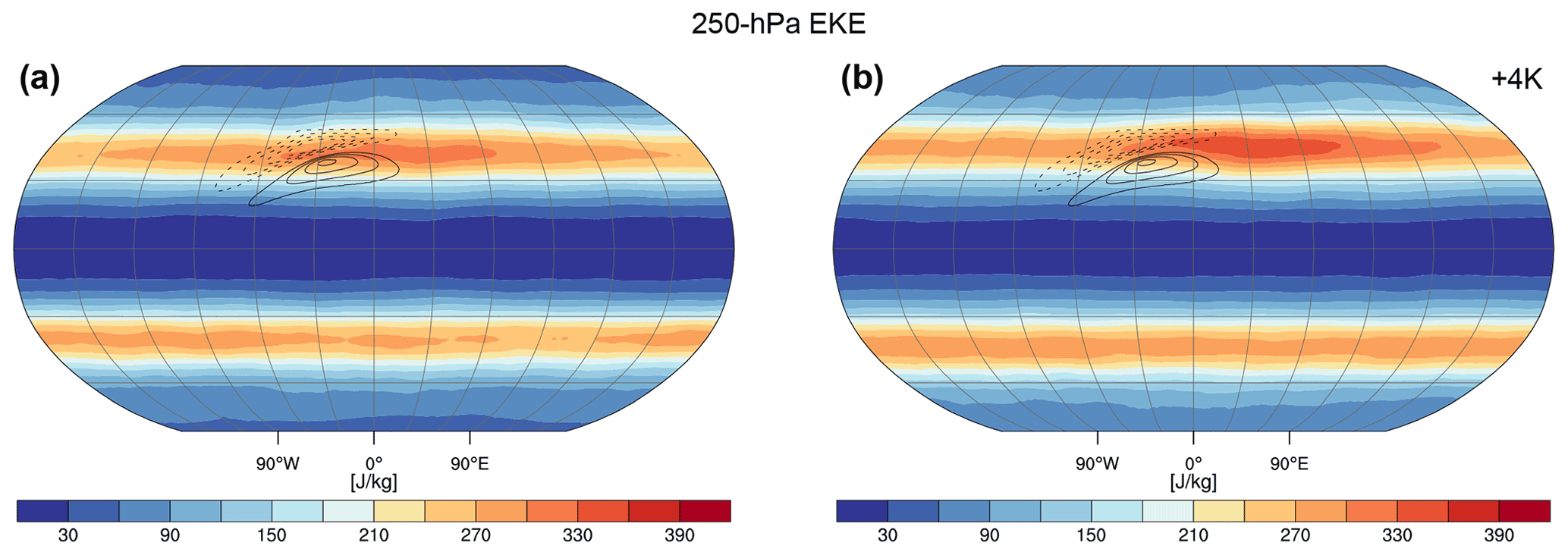
Figure 1 Eddy kinetic energy (shading; J kg⁻¹) at the 250 hPa level for the (a) Qobs control run with SST front in the Northern Hemisphere and (b) with homogeneous warming by 4 K at the surface. The SST front is indicated in this and the following figures by its imprint in the 2 m temperature after removing the zonal mean (black solid contours indicate positive values and dashed negative values; starting at ±0.5 K in steps of 0.5 K).

The aquaplanet's atmosphere is initialized with a standard configuration set: the atmosphere following the equations given by the Jablonowski–Williamson baroclinic wave test case (Jablonowski and Williamson, 2006) and the background SST following the well-known “Qobs” distribution by Neale and Hoskins (2001), which approximates the observed zonal mean SST distribution. In the Northern Hemisphere, an idealized SST front is superposed on the “Qobs” distribution. This SST front consists of two ellipsoids of the same size but reversed sign. The maximum amplitude at the centers of the ellipsoids is 10 K, decaying exponentially with distance. The mid-point between the two ellipsoids is placed at 30^∘ W and 42^∘ N, and their centers are shifted against each other by 7^∘ latitude. Finally, the ellipsoids are rotated by 25^∘ with respect to a longitude circle, and the minimum temperature is limited to the freezing temperature of 273.15 K. By imposing rotated positive and negative SST anomalies, we mimic the combined effect of the Gulf Stream and the land–sea contrast in the western North Atlantic. No SST front is placed in the Southern Hemisphere to allow for a direct comparison with a front-free zonally symmetric atmosphere. The zonally symmetric background SST profile, the SST front, and the 2 m temperature anomaly computed as deviation from the zonal mean of the climatological 2 m temperature are shown in Fig. A1. The 2 m temperature anomaly will be shown in each figure throughout the paper (see for example solid and dashed contours in Fig. 1).

Two simulations are performed: one following the setup as just described and one with a uniform increase in the SST of 4 K. For each simulation, the model is spun up for a month, and then a total of 20 winter seasons are simulated, corresponding to 60 simulated perpetual months. Note that there is no seasonality in the model, and the solar zenith angle at the Equator at noon is kept at constant 90^∘.

2.2 Eddy kinetic and eddy available potential energy budget

To understand the change in eddy kinetic energy (EKE) and eddy available potential energy (EAPE), tendencies for EKE and EAPE are computed using the equations already used in Chang et al. (2002), Drouard et al. (2015), Rivière et al. (2018), Schemm and Schneider (2018), and Schemm and Rivière (2019), which go back to the work by Cai and Mak (1990) and Orlanski and Katzfey (1991).

2.2.1 Eddy kinetic energy equation

The EKE and EAPE budget have been derived before and are presented here for completeness. The EKE budget equation is obtained by high-pass filtering of the primitive equations of motion in pressure coordinates and after multiplication by the high-pass-filtered horizontal wind components. A 10 d frequency cutoff is used in the high-pass filter. The resulting tendency equation, where primes denote high-pass-filtered quantities and overbars low-pass-filtered quantities, is

$$\begin{array}{}\text{(1)}& \begin{array}{rl}{\displaystyle \frac{\partial K_{\mathrm{e}}^{\prime }}{\partial t}}& =-\mathrm{\nabla }\cdot \left(\mathit{v}{K}_{\mathrm{e}}^{\prime }+{\mathit{v}}_{\mathrm{a}}^{\prime }{\mathit{\varphi }}^{\prime }\right)-{\displaystyle \frac{\partial }{\partial p}}\left(\mathit{\omega }{K}_{\mathrm{e}}^{\prime }+{\mathit{\omega }}^{\prime }{\mathit{\varphi }}^{\prime }\right)\\ & +{\mathit{\omega }}^{\prime }{\displaystyle \frac{\partial {\mathit{\varphi }}^{\prime }}{\partial p}}-{\mathit{v}}^{\prime }\cdot \left({\mathit{v}}_{\mathrm{3}}^{\prime }\cdot \mathrm{\nabla }\stackrel{\mathrm{‾}}{\mathit{v}}\right)+R_{K_{\mathrm{e}}},\end{array}\end{array}$$

where the residual term is $R_{K_{\mathrm{e}}}={\mathit{v}}^{\prime }\cdot \left(\stackrel{\mathrm{‾}}{{\mathit{v}}_{\mathrm{3}}\cdot \mathrm{\nabla }\mathit{v}}-{\stackrel{\mathrm{‾}}{\mathit{v}}}_{\mathrm{3}}\cdot {\mathrm{\nabla }}_{\mathrm{3}}\stackrel{\mathrm{‾}}{\mathit{v}}\right)$, and ϕ^′ is the filtered geopotential height. Three-dimensional vectors have a subscript “3”. The sum of the three terms $-\frac{\partial }{\partial p}\left({\mathit{\omega }}^{\prime }{\mathit{\varphi }}^{\prime }\right)+{\mathit{\omega }}^{\prime }\frac{\partial {\mathit{\varphi }}^{\prime }}{\partial p}-\mathrm{\nabla }\left({\mathit{v}}_{\mathrm{a}}^{\prime }{\mathit{\varphi }}^{\prime }\right)$, where ${\mathit{v}}_{\mathrm{a}}^{\prime }$ is the ageostrophic wind, denotes the pressure gradient force ($-{\mathit{v}}^{\prime }\cdot \mathrm{\nabla }{\mathit{\varphi }}^{\prime }$). The first term on the right-hand side denotes the flux horizontal convergence of EKE, the second the horizontal ageostrophic geopotential flux, and the third and fourth terms the corresponding vertical fluxes. The fifth term is the internal baroclinic conversion from EAPE to EKE and the sixth term the barotropic conversion. The last term, finally, is the residual accounting for numerical errors in the computation of the EKE budget. If the time mean is used instead of a high-pass filter, the equation reduces to the EKE tendency of Orlanski and Katzfey (1991). More details on the derivation are presented in the Appendix of Schemm and Rivière (2019).

2.2.2 Eddy available potential energy equation

Similarly, an equation for the EAPE tendency is obtained by multiplying the high-pass-filtered thermodynamic equation with ${\mathit{\theta }}^{\prime }/S$ (Chang et al., 2002; Drouard et al., 2015), which yields

$$\begin{array}{}\text{(2)}& \begin{array}{rl}{\displaystyle \frac{\partial P_{\mathrm{e}}^{\prime }}{\partial t}}& =-\mathrm{\nabla }\cdot \left(\mathit{v}{P}_{\mathrm{e}}^{\prime }\right)-{\mathit{\omega }}^{\prime }{\displaystyle \frac{\partial {\mathit{\varphi }}^{\prime }}{\partial p}}-{\displaystyle \frac{\mathrm{1}}{S}}{\mathit{\theta }}^{\prime }\left({\mathit{v}}^{\prime }\cdot \mathrm{\nabla }\stackrel{\mathrm{‾}}{\mathit{\theta }}\right)\\ & -{\displaystyle \frac{\mathrm{1}}{S}}{\displaystyle \frac{\partial }{\partial p}}\left(\mathit{\omega }{\displaystyle \frac{{\mathit{\theta }}^{\prime \mathrm{2}}}{\mathrm{2}}}\right)+{\displaystyle \frac{\mathrm{1}}{S}}{\mathit{\theta }}^{\prime }{Q}^{\prime }+R_{P_{\mathrm{e}}},\end{array}\end{array}$$

where the residual term is $R_{P_{\mathrm{e}}}=\frac{{\mathit{\theta }}^{\prime }}{S}\left[\stackrel{\mathrm{‾}}{\left({\mathit{v}}_{\mathrm{3}}\cdot \mathrm{\nabla }\mathit{\theta }\right)}-{\stackrel{\mathrm{‾}}{\mathit{v}}}_{\mathrm{3}}\cdot {\mathrm{\nabla }}_{\mathrm{3}}\stackrel{\mathrm{‾}}{\mathit{\theta }}\right]$. The diabatic source term is denoted by Q^′ and includes short- and longwave radiation $Q_{\mathrm{RD}}^{\prime }$, parameterizations of convection $Q_{\mathrm{CN}}^{\prime }$, turbulence $Q_{\mathrm{TR}}^{\prime }$, microphysics $Q_{\mathrm{MP}}^{\prime }$, and a resolved-scale saturation adjustment scheme that produces condensation and evaporation $Q_{\mathrm{SA}}^{\prime }$. The saturation adjustment is called before and after the dynamical core in the model. Their contributions to the build-up of EAPE will be discussed in detail in this study. The tendencies from gravity wave drag, which are small, are neglected, and the tendencies from sub-grid-scale orography do not exist on an aquaplanet. The static stability parameter is defined as $S=-h^{-\mathrm{1}}\frac{\partial {\mathit{\theta }}_R}{\partial p}$. The definition makes partial use of quasi-geostrophic scaling assumptions and of a vertical reference potential temperature computed from the climatological mean of the simulation. The scale height is $h=\frac{R}{p}{\left(\frac{p}{p_{\mathrm{0}}}\right)}^{R/c_p}$. The second term on the right-hand side is the internal baroclinic conversion from EAPE into EKE – the same as in Eq. (1) but with opposite sign – the third term is the external baroclinic conversion representing the conversion of mean available potential energy into EAPE, and the fourth term is the vertical flux convergence. The last term again denotes the residual. The analysis in the following sections puts its emphasis on the conversion terms rather than on advection and ageostrophic geopotential flux. The latter only redistribute energy and are not global sources and sinks.

The external baroclinic conversion into EAPE is the scalar product between the eddy heat flux and the mean baroclinicity. It can be decomposed into contributions from the mean baroclinicity; the eddy total energy $T_{\mathrm{e}}^{\prime }$, which is given by the sum of EAPE and EKE; and the baroclinic conversion efficiency (Rivière et al., 2018),

$$\begin{array}{}\text{(3)}& {\displaystyle \frac{\mathrm{1}}{S}}{\mathit{\theta }}^{\prime }\left({\mathit{v}}^{\prime }\cdot \mathrm{\nabla }\stackrel{\mathrm{‾}}{\mathit{\theta }}\right)=T_{\mathrm{e}}^{\prime }\mathrm{|}{\mathit{B}}_{\mathrm{s}}\mathrm{|}{E}_{\mathrm{ff}},\end{array}$$

where the eddy efficiency E_ff is defined as

$$\begin{array}{}\text{(4)}& E_{\mathrm{ff}}={\displaystyle \frac{\mathrm{|}{\mathit{Q}}_{\mathrm{s}}\mathrm{|}}{T_{\mathrm{e}}^{\prime }}}\cos \left({\mathit{Q}}_{\mathrm{s}},{\mathit{B}}_{\mathrm{s}}\right),\end{array}$$

where${\mathit{Q}}_{\mathrm{s}}=\frac{\mathrm{1}}{\sqrt{S}}\left({\mathit{v}}^{\prime }{\mathit{\theta }}^{\prime }\right)$ is the eddy heat flux normalized by the static stability and ${\mathit{B}}_{\mathrm{s}}=-\frac{\mathrm{1}}{\sqrt{S}}\mathrm{\nabla }\stackrel{\mathrm{‾}}{\mathit{\theta }}$ is the background baroclinicity. The eddy efficiency is independent of the eddy amplitude and thus, in contrast to the eddy heat flux, particularly useful for the study of baroclinic conversion changes. The efficiency is maximized if the magnitude and orientation of the vertical westward tilt with height are such that the resulting eddy heat flux (Q_s) aligns with the mean baroclinicity B_s (see Fig. 1 in Schemm and Rivière, 2019). Notably, the time mean of the eddy efficiency relates to the eddy diffusivity in storm tracks (Eq. 9 in Schemm and Rivière, 2019), which is known to control the amplitude and meridional transport characteristics of baroclinic eddies (Held and Larichev, 1996; Lapeyre and Held, 2003; Schemm and Schneider, 2018).

2.3 Feature-based cyclone tracking

The feature-based method to detect surface cyclones is based on a contour search approach as introduced by Wernli and Schwierz (2006). The scheme identifies local minima in the sea level pressure field (SLP), which are enclosed by a closed SLP contour. Subsequently, these minima are tracked in time at 6-hourly temporal resolution. As in previous studies, the minimum lifetime of a track is 1 d. Further refinements related to splitting and merging of tracks that extend the original scheme are described in Sprenger et al. (2017). These refinements do not affect the results of this study. The total number of analyzed cyclone tracks from the 20 simulated winter seasons is about 15 900 in the control simulation and 13 500 in the warmed simulation.

The identified surface tracks are used to study deepening rates, which are defined as the change of SLP along a track computed between two consecutive 6-hourly time steps. Additionally considered are maximum intensities, defined as the minimum SLP value found along a track, and the lifetime and meridional displacements. The latter is defined once as the difference in latitude between genesis and lysis (corresponding to the first and last time steps along a track, respectively) and the difference between the genesis latitude and the latitude of maximum intensity.

3 Results

3.1 Storm track response to warming on aquaplanet compared with CMIP5 data

The SST front on the aquaplanet anchors a locally enhanced storm track that extends from slightly upstream of the center of the front near 30^∘ E downstream toward 90^∘ E (Fig. 1a and b). Further downstream near 150^∘ E, 250 hPa EKE values begin to decrease and approach those found in the undisturbed Southern Hemisphere. EKE begins to strengthen again near 150^∘ W. Near 30^∘ N, 30^∘ E there is an indication of the formation of a stationary trough, as predicted by theory, because the midlatitude atmosphere tends to offset low-level warming by horizontal advection of cold air from the north, which requires the presence of a low-pressure anomaly located downstream of the heat source (Hoskins and Karoly, 1981). Aside from this slight trough anomaly, the storm track appears zonally symmetric, as would be expected on an aquaplanet. We note that the overall patterns are also similar on different levels, such as the 500 hPa level but with a reduced magnitude. Overall, the simulated interactions between the idealized SST front and the extratropical circulation result in a local intensification of the EKE that affects the entire depth of the troposphere and extends far downstream of the SST front. The response of this storm track downstream of the SST front to idealized global warming is the focus of the following analysis.

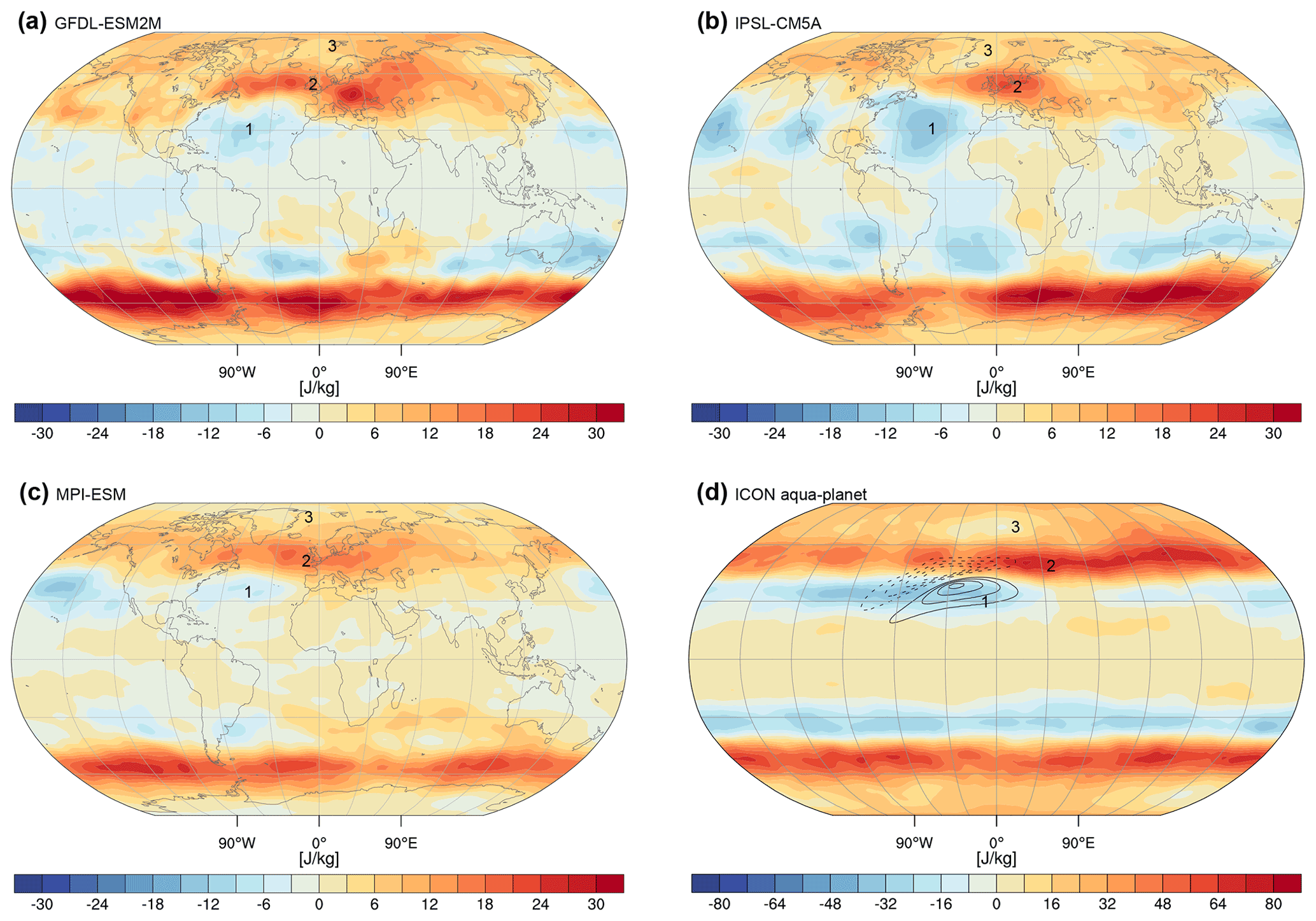
Figure 2 Eddy kinetic energy difference (shading; J kg⁻¹) at the 250 hPa level between the periods 2091–2100 and 2011–2030 (December–February) for the RCP8.5 scenario and for the (a) GFDL-ESM2M, (b) IPSL-CM5A LR, (c) MPI-ESM LR, and (d) idealized ICON aquaplanet simulation including a SST front in the Northern Hemisphere, which is warmed by 4 K.

The 250 hPa EKE change between the control scenario and the warming scenario, consisting of a simple uniform surface warming of 4 K, shows three distinct anomaly patterns that are also found in fully coupled CMIP5 simulations under the RCP8.5 greenhouse gas emission scenario. The EKE change at the end of the century under the RCP8.5 scenario compared to present-day conditions (Fig. 2) shows a poleward shift and intensification of the storm track in the Southern Hemisphere, which has been documented in previous literature (Chang et al., 2012). While the magnitude of the EKE change differs among the models selected here, the pattern does not qualitatively change when all models and all ensemble members are included (see Fig. 1 in Tamarin and Kaspi, 2017); the overall pattern of EKE changes exhibits similarities. For example, EKE decreases over the North Atlantic equatorward of the Gulf Stream SST front (labeled “1” in Fig. 2), while it increases downstream and northeastward of the SST front (labeled “2” in Fig. 2). In addition, a local minimum in EKE increase is observed poleward of the SST front (labeled “3” in Fig. 2). These features are all reproduced in the idealized aquaplanet simulation (see corresponding labels in Fig. 2d). Furthermore, it is interesting to note that these features are also present on the aquaplanet in the jet stream as represented by 300 hPa wind speeds (Fig. D1a) and agree with the flow modification by changes in stationary waves (Fig. D1b). In the Southern Hemisphere, the storm tracks on the aquaplanet shift poleward and tend to intensify. In the Northern Hemisphere and downstream of the idealized SST front, EKE increases, while further poleward and equatorward EKE decreases (see corresponding labels in Fig. 2d). Taken together, the pattern of EKE changes in the aquaplanet simulation downstream of and at the idealized SST front is reminiscent of the changes projected by the more complex Earth system models.

In contrast to the Gulf Stream SST front, the EKE change over the Kuroshio front is less pronounced (Fig. 2a, b, and c). Possibly, this is related to climatologically weaker SST gradients over the western North Pacific, a more zonal orientation of the SST front and the jet stream, and the distance of the SST front from the continent. Nevertheless, we note that the change pattern is also not absent. The stronger signal over the North Atlantic suggests that likely other mechanisms are at play, including changes to stationary waves induced by topography (Wills et al., 2019) and the jet stream (Harvey et al., 2020), as well as the formation of the North Atlantic warming hole. The North Atlantic warming hole describes the counterintuitive cooling of the SSTs of the northern North Atlantic in simulations of global warming (Keil et al., 2020). This regional SST cooling has been shown to contribute to locally enhanced near-surface baroclinicity and stronger downstream EKE and eddy momentum convergence (Gervais et al., 2018). However, the aquaplanet simulation shows that the presence of an SST front alone is sufficient to simulate a response of the storm tracks to warming, similar to that found over the North Atlantic in CMIP simulations. In what follows, we focus our analysis on the mechanisms that lead to the intensification of the storm track downstream of the idealized SST front. This focus does not imply that the North Atlantic warming hole is not an important factor affecting the net response of the North Atlantic storm track to global warming, nor does it mean that the mechanisms causing the response on the aquaplanet are the same as those causing the response in CMIP simulations.

3.2 Detailed analysis of the EAPE budget

In the following, we consider the change in EAPE between the +4 K warmed and control simulations, since the EAPE changes may eventually precede those in EKE in both time and space. Unless stated otherwise, fields shown in the following are mass-weighted vertically averaged between 1000–200 hPa.

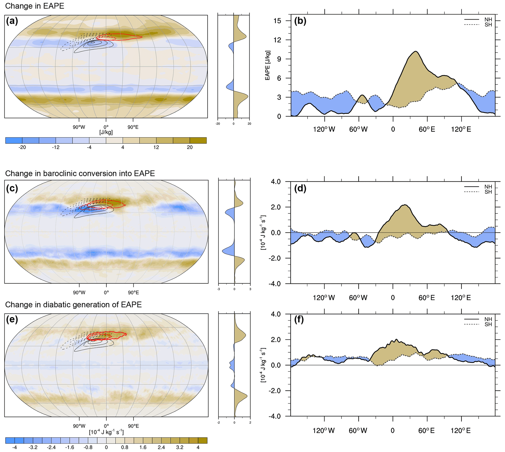
Figure 3 (a) EAPE difference between warmed and control simulations (mass-weighted vertically averaged between 1000–200 hPa). Additional red contours indicate selected EAPE value of 90 J kg⁻¹ in the control (red dashed) and warmed (red solid) simulations; (c) change in external baroclinic conversion and (e) diabatic generation rates of EAPE. Additional red contours in (c) and (e) indicate 8 × 10⁻⁴ J (kg s)⁻¹ in the control (red dashed) and warmed (red solid) simulations. (b) EAPE difference between the warmed and control simulations but meridionally averaged over the Northern Hemisphere (solid) and Southern Hemisphere (dashed) midlatitudes (20–60^∘ N). Color shading highlights differences between the two hemispheres. (d, f) As (b) but for external baroclinic and diabatic EAPE generation.

The poleward shift of the zone with the highest EAPE is clearly seen in both hemispheres from the difference of EAPE between both simulations (shading in Fig. 3a). Further, there is a clear increase in the EAPE magnitude downstream and northeast of the SST front and an eastward expansion of the region with enhanced EAPE. These changes are not found at any other latitude or longitude (red contours in Fig. 3a). The increase is most pronounced at levels above 500 hPa and largest at 300 hPa, while at 700 hPa and below there is a mild to no decrease in EAPE (not shown). Finally, there is a local reduction of EAPE poleward of the SST front such that the changes in EAPE show a tripole pattern that is qualitatively similar to that of EKE (cf. Figs. 3a and 2d). Considering the zonal mean of the vertically averaged difference shows that EAPE decreases within a band between 30 and 45^∘ N but increases poleward of 45^∘ N with a peak at 55^∘ N. Furthermore, there is a locally reduced increase between 60–70^∘ N and another enhanced increase near the poles north of 75^∘ N in both hemispheres (Fig. 3a).

The differences between both hemispheres are visible in the meridional mean changes of external baroclinic conversion (Fig. 3b). For the Northern Hemisphere, the difference between the meridional means of both simulations shows an EAPE increase between 0–120^∘ E, which is well above the increase seen in the Southern Hemisphere (black dashed contour in Fig. 3b). Further downstream and upstream, between 120–180^∘ E and 180–0^∘ W, meridionally averaged EAPE in the warmed simulation is only marginally larger compared to the control simulation (black solid contour in Fig. 3b). However, it is smaller compared to the increase observed in the Southern Hemisphere. This suggests less eddy activity far up- and downstream of the SST front compared to storm tracks that form in the absence of a SST front.

To summarize, the changes in the Southern Hemisphere (black dashed contour in Fig. 3b) indicate that EAPE not only shifts poleward in the warmer climate but increases at nearly all longitudes, which appears to be due to the increase in EAPE everywhere poleward from 45^∘ N toward the poles (Fig. 3b), while in the Northern Hemisphere the increase is confined but clearly increased downstream of the SST front.

Next, consideration is given to the two leading source terms of EAPE, which are the external baroclinic conversion and diabatic EAPE generation. The maximum EAPE generation by external baroclinic conversion occurs northeast of the SST front (Fig. 3c). As for EAPE, the maximum in external baroclinic conversion is shifted northeastward relative to the SST front (Fig. 3c), and the absolute values clearly increase in the warmed simulation (red contours in Fig. 3c). The difference between the meridionally averaged midlatitude (20–60^∘ N) external baroclinic conversion rates shows a clear increase between 30^∘ W –90^∘ E in the Northern Hemisphere (Fig. 3d), which is most pronounced downstream of the SST front between 30^∘ W–60^∘ E. It agrees well with the EAPE change (Fig. 3b). In fact, the peak is slightly upstream of the increase in EAPE, indicating the importance of EAPE advection. At all other longitudes, the meridionally averaged external baroclinic conversion in the Northern Hemisphere (NH) is reduced (solid contour in Fig. 3d) relative to the control as well as relative to the change in the Southern Hemisphere (SH, blue shading in Fig. 3d). In fact, in the Southern Hemisphere, the difference in the meridionally averaged conversion fluctuates around zero (dashed contour in (Fig. 3d), indicating that the poleward shift of the external baroclinic conversion in the warmer climate is not accompanied by an increase in the external baroclinic conversion (this also holds true if the conversion rate is meridionally averaged over the entire hemisphere instead of midlatitudes only). However, in the zonal mean the change in external baroclinic conversion shows a dipole structure akin to the shift of the storm track. The positive and negative peaks largely cancel each other. This implies that the northern hemispheric local increase in external baroclinic conversion downstream of the SST front is largely balanced by a decrease elsewhere at the same longitude. Consequently, the local increase in EAPE downstream of the SST front is partly explained by increased external baroclinic conversion, but the global increase in EAPE seen in Fig. 3a, b is not.

Before turning attention to the diabatic EAPE generation, we take a closer look at the baroclinic conversion changes near the SST front. External baroclinic conversion into EAPE is the product between the eddy total energy, the mean baroclinicity, and the conversion efficiency. In response to the imposed uniform surface warming, the mean baroclinicity shifts poleward (black contours in Fig. 4). The shift in the SH is mostly symmetric, while in the NH the poleward increase in mean baroclinicity is zonally limited to an elongated band extending from upstream of the SST front to approximately 120^∘ E, while there is no increase further downstream. At the same time, there is a reduction up- and downstream of the warm side of the front but only a reduced weakening in the direct vicinity downstream of the SST front, where there is a local increase in conversion efficiency. Eddy total energy, the sum of EKE and EAPE, increases as expected downstream and to the northeast of the SST front, indicating the stronger storm track (red contours in Fig. 4). Much of the local change in external baroclinic conversion is dictated by local changes in the conversion efficiency (shading in Fig. 4), which increases poleward of the SST front but in particular to the northeast and downstream of it (asterisk in Fig. 4), while it decreases upstream and to the south. As a result, in region 2 the external baroclinic conversion increases at all analyzed levels above 500 hPa, while there is a weakening below 700 hPa (not shown), and it decreases in region 1. Furthermore, in region 3, the local minima in EAPE and EKE imply a reduction of eddy total energy, which combined with reduced eddy efficiency results in moderately reduced external baroclinic conversion in this region.

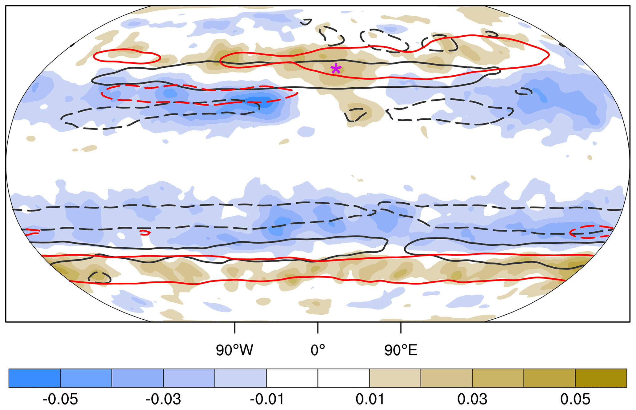
Figure 4 Change in external baroclinic conversion efficiency (shading), eddy total energy (red; ±25​​​​​​​ J kg), and background baroclinicity (black contours; dashed indicate negative and solid positive values; units of ±1.5 × 10⁻⁶ s⁻¹). All fields are mass-weighted vertically averaged between 1000–200 hPa. The key region of enhanced conversion efficiency downstream of the SST front is marked by an asterisk.

Hence, we conclude that as the external baroclinic conversion does not change globally, the SST front in the first place acts to localize the external baroclinic conversion downstream of the front. This localization is such that in the warmer climate, external baroclinic conversion efficiency increases northeast of the SST front. This indicates a better alignment of the eddy heat flux with the mean baroclinicity compared to the control. As a consequence, the eddies become more efficient in tapping into the mean potential energy reservoir.

The second main EAPE source term is the diabatic generation. The change of the net diabatic EAPE generation, which in absolute terms is strongest near the SST front (red contour in Fig. 3e), also indicates a poleward shift in both hemispheres (Fig. 3e). The difference between the meridional means indicates an increase in the NH near the front (solid contour in Fig. 3f) that exceeds the increase in the SH at the same longitude (brown shading in Fig. 3f). However, at other longitudes, the increase in the meridional mean is generally weaker in the NH compared to the SH (east of 100^∘ E and west of 50^∘ W; Fig. 3f). This is further underlined by comparing the meridionally averaged changes in the two hemispheres, which are positive almost everywhere (see dashed and solid contours in Fig. 3f). Consequently, the zonal means are positive poleward of 45^∘ N and 45^∘ S and mostly symmetric between the two hemispheres. Hence, we conclude that globally the increase in EAPE (Fig. 3b) is primarily explained by enhanced diabatic generation of EAPE.

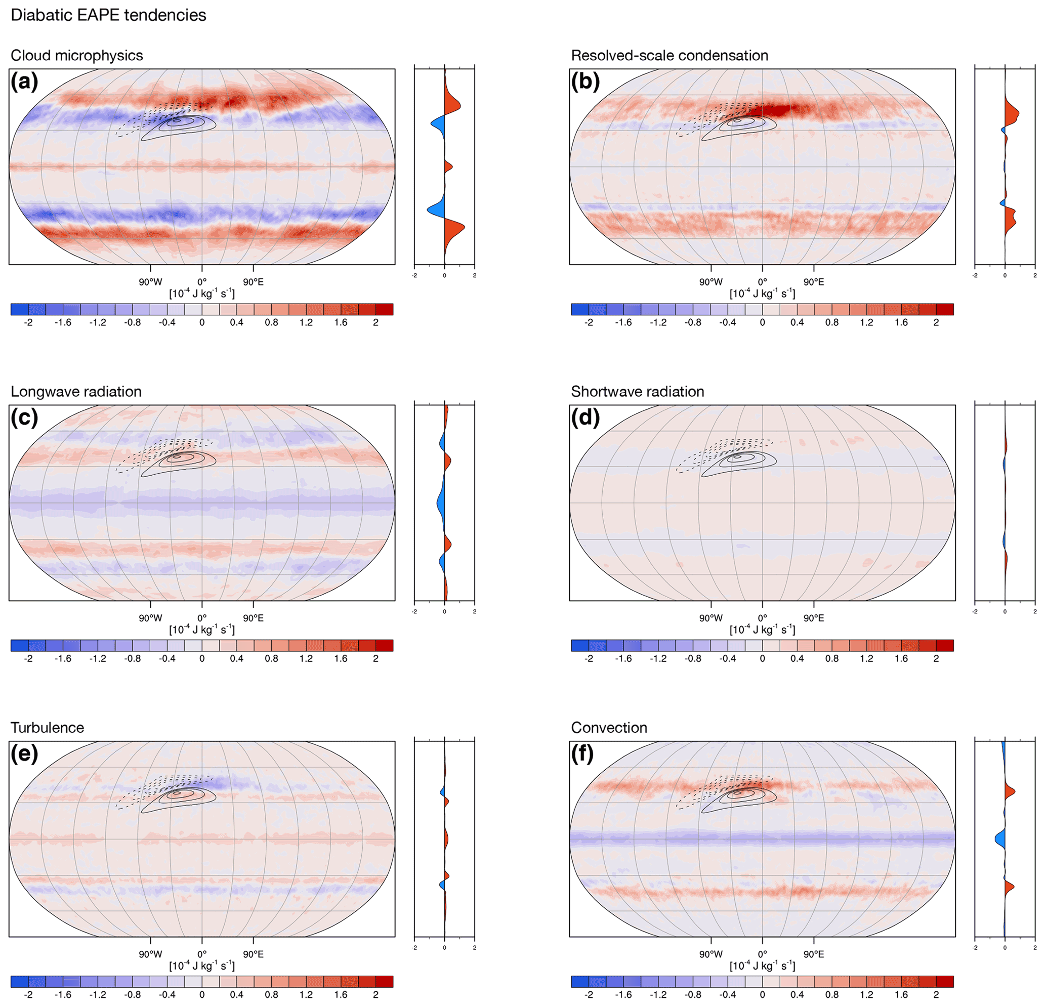
Figure 5 Mass-weighted vertically averaged change of different diabatic EAPE tendencies between the warmed and control simulations due to (a) cloud microphysics, (b) saturation adjustment, (c) longwave and (d) shortwave radiation, (e) turbulence, and (f) parameterized convection (color shading). Vertical averages are taken between 1000–200 hPa.

In the following, the diabatic EAPE generation is partitioned into the contributions of different diabatic processes (Fig. 5). Even though the diabatic EAPE generation depends on the underlying model, the sub-grid-scale parameterizations, and their specific design, a decomposition of the diabatic EAPE tendency is still of scientific merit as it points towards the dominant physical processes accounting for the changes. The strongest increase results from the resolved-scale condensation and the cloud microphysics scheme, which simulates in-cloud phase changes of water, such as ice formation and sublimation (Fig. 5a). In the NH there is a clear increase in diabatic generation of EAPE by microphysical processes north of the front. This increase extends from upstream near 90^∘ W of the front and downstream to 120^∘ E. However, the zonal mean indicates that much of the increase is globally compensated for by a decrease further equatorward. In contrast, the change in resolved-scale condensation and evaporation, i.e., due to saturation adjustment, is of similar importance near the SST front in terms of magnitude, and the absence of a clear dipole structure in the zonal mean indicates no compensation elsewhere (Fig. 5b).

The diabatic EAPE tendencies from the other processes are considerably smaller. EAPE longwave radiation tendencies change sign at different levels (Fig. C1). At the 700 and 500 hPa levels EAPE tendency from longwave radiation is positive, which are levels where the cloud base is warmed from thermal radiation received from the Earth surface (Fig. C1). Thus, in the vertically averaged framework, the positive and negative anomalies in Fig. 5c result not only from a poleward shift but also from an enhancement of the existing positive and negative patterns originating from different vertical levels. Nevertheless, the magnitude is considerably smaller compared to that of cloud physics and condensation, and the zonal mean suggests only little global change. In contrast to the longwave radiation, the EAPE tendencies from shortwave radiation partly oppose longwave radiation at upper levels. In general the shortwave EAPE tendencies are close to zero in the lower levels of the troposphere (e.g., 700 hPa), while they are positive in the upper troposphere (e.g., 300 hPa), thereby partially counteracting the negative longwave tendencies (Fig. C1). EAPE generation by turbulence is negative north of the front and positive south of it, weakening with height (Fig. 5e). Turbulence contrasts with EAPE tendencies from parameterized convection, which includes turbulent mixing in convective plumes and latent heating. Convective EAPE generation increases at the SST front (Fig. 5f) and poleward of the maximum in the control run (Fig. C1b), with no concurrent and well-marked reduction equatorward (Fig. 5f).

In summary, the local increase in external baroclinic conversion rates dominates the strong local increase in EAPE downstream of the SST front with only a smaller contribution from diabatic EAPE production, which is slightly increased near the SST front. The global EAPE increase, however, is the result of increased diabatic EAPE production in the first place due to resolved-scale condensation.

3.3 Detailed analysis of the EKE budget

Following the discussion of the EAPE budget, this section discusses the EKE change shown in Fig. 6a, the budget, and related changes. The EKE change in the NH exhibits a strong asymmetry between the region upstream and downstream of the SST front (Fig. 6b). In the SH, EKE is solely shifted poleward with no notable increase. The two main EKE source terms are the internal baroclinic conversion, which converts EAPE into EKE (third term on the right-hand side in Eq. 6), and the barotropic conversion (fourth term on the right-hand side in Eq. 6), which generates EKE from the low-frequency background flow. The ageostrophic geopotential fluxes and advection are not discussed as both processes are not global EKE sources or sinks but redistribute EKE locally.

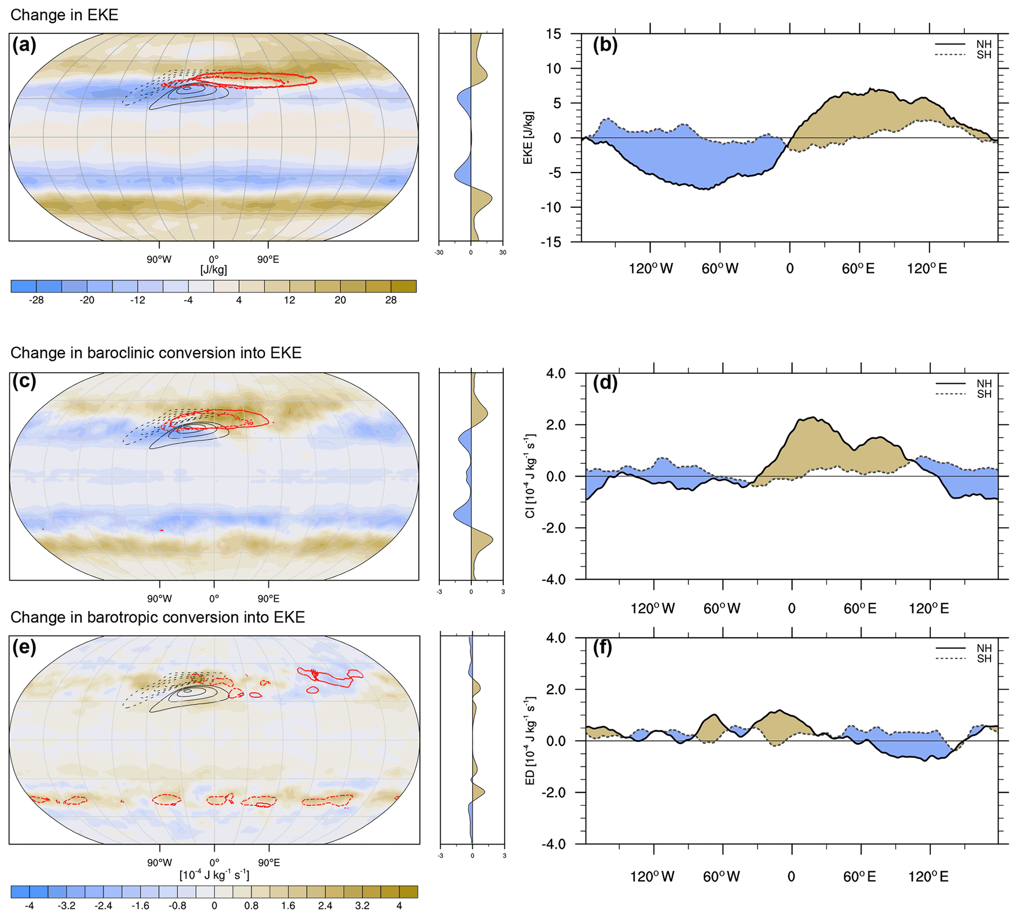
Figure 6 (a) EKE difference between warmed and control simulations (mass-weighted vertically averaged between 1000–200 hPa). Additional red contours indicate the selected EKE value of 135 J kg⁻¹ in the control (red dashed) and warmed (red solid) simulations; black contours indicate the SST front. (c) Change in internal baroclinic and (e) barotropic generation rates of EKE. Additional red contours in (c) indicate 12 × 10⁻⁴ J (kg s)⁻¹ in the control (red dashed) and warmed (red solid) simulations and in (e) indicate −3 × 10⁻⁴ J (kg s)⁻¹ (note that the time-mean barotropic conversion is mostly negative). (b) EKE difference between the warmed and control simulations but meridionally averaged over the Northern Hemisphere (solid) and Southern Hemisphere (dashed) midlatitudes (20–60^∘). Color shading highlights differences between the two hemispheres. (d, f) As (b) but for baroclinic and barotropic EKE generation.

The vertically averaged time-mean barotropic conversion is mostly negative in our simulations (not shown) and acts as an EKE sink as is generally the case within storm tracks (Chang et al., 2002). The change in EKE, shown in Fig. 6a, displays the aforementioned tripole with an EKE decrease equatorward and upstream of the SST front's center, an increase poleward and downstream, and a slight reduction at the longitude of the SST front's center but at high latitudes (at 70^∘ N, 30^∘ W in Fig. 6a). The meridionally averaged (20–60^∘) change in EKE is close to zero for the SH (dashed contour in Fig. 6b), which once again indicates that the SH experiences a poleward shift with no marked increase in EKE in the midlatitudes. EKE increases if averaged over the entire extratropics (20–90^∘), but this increase is dominated by EKE at polar latitudes with no to little change in midlatitudes. In the NH, EKE reduces upstream and equatorward of the front between 0 and 180^∘ and increases downstream and poleward of the front (red solid contour in Fig. 6a). The storm track hence shifts poleward and becomes weaker upstream of the front relative to the control run and stronger downstream of the front.

As is the case for external baroclinic EAPE generation, there is a distinct increase in internal baroclinic generation of EKE (Fig. 6c). The increase in internal baroclinic conversion into EKE starts, similarly to external baroclinic conversion into EAPE, upstream of the front, reaches a first maximum near 25–30^∘ W, and continues to be increased downstream with a second maximum near 60^∘ W, which is best seen in the meridional average (Fig. 6d). The increase exceeds the change seen in the SH. Further downstream and around the dateline, baroclinic conversion into EKE is reduced compared to the levels seen in the SH. In addition, internal baroclinic conversion is slightly reduced poleward of the SST front. Overall, the change in the meridionally averaged internal baroclinic conversion is small in the SH, indicating a poleward shift with only a minor net increase (the dashed line in Fig. 6d is mostly above the zero contour). The change in the barotropic tendency, which is climatologically negative, is positive in the area of and slightly upstream from the SST front (20^∘ W–5^∘ E), indicating a lower barotropic EKE sink in this area. Downstream, between 60–150^∘ W, the negative barotropic EKE tendency is increased, which indicates enhanced transformation of EKE to zonal mean kinetic energy. For the SH, the meridional average of the change is close to zero, indicating a poleward shift with no marked change in amplitude. To summarize, as for EAPE it is primarily the internal baroclinic conversion from EAPE into EKE that is the key source term underlying the observed tripolar pattern of EKE change.

3.4 Change in stationary waves and local EKE–EAPE redistribution

Topography, land–sea thermal contrasts, diabatic heating associated with eddies, and eddy heat and momentum fluxes lead to the formation of stationary waves (Held et al., 2002). Previous idealized aquaplanet studies with localized SST anomalies have shown that stationary waves tend to strengthen storm tracks in their entry region and weaken them in their exit region (Kaspi and Schneider, 2011, 2013). Here, we consider departures of 500 hPa geopotential from the zonal mean as a proxy for stationary waves. Anomalies relative to the control simulation suggest the existence of a strengthened trough located about 90^∘ downstream and 15–20^∘ poleward of the SST front, as well as a strengthened stationary ridge shifted downstream by another 90^∘ (green contours in Fig. D1b). Upstream of the stationary trough, anomalous equatorward EAPE–EKE advection contributes to the local decrease in EAPE–EKE at polar latitudes (region “3” in Fig. 2). This indicates that in addition to weakened internal and external baroclinic conversions, eddy-mean-flow feedbacks via changes of stationary wave patterns contribute to the reduction of storm track activity in region 3 via changes in EAPE and EKE advection. Further downstream, enhanced poleward EAPE–EKE advection between the stationary trough and the ridge locally increases EKE between 60^∘ N, 90–120^∘ E relative to all other longitudes. As shown below, using feature-based cyclone tracking, the transition zone between the stationary trough and ridge marks the exit region of the surface storm track (in agreement with Kaspi and Schneider, 2011, 2013).

4 Change in characteristics of extratropical cyclones from feature-based tracking

In the following section, consideration is given to the changes in several life cycle characteristics of extratropical cyclones obtained from a featured-based surface cyclone tracking. The total number of analyzed cyclone tracks from the 20 winter seasons is approximately 15 900 in the control simulation and 13 500 in the warmed simulation, corresponding to a reduction by approximately 15 %, which is in agreement with earlier studies (Sinclair et al., 2020).

4.1 Change in cyclone frequency

The cyclone frequency indicates the relative proportion of all time steps at which a grid point is affected by a surface cyclone. The frequency is climatologically high in regions where cyclones are in their mature phase (and cover a wide area) and in regions where the propagation speed is low (they affect the same region during several time steps). Such regions are typically located downstream and poleward of high-EKE regions. High EKE indicates regions of high cyclone intensity and propagation speed (Schemm and Schneider, 2018).

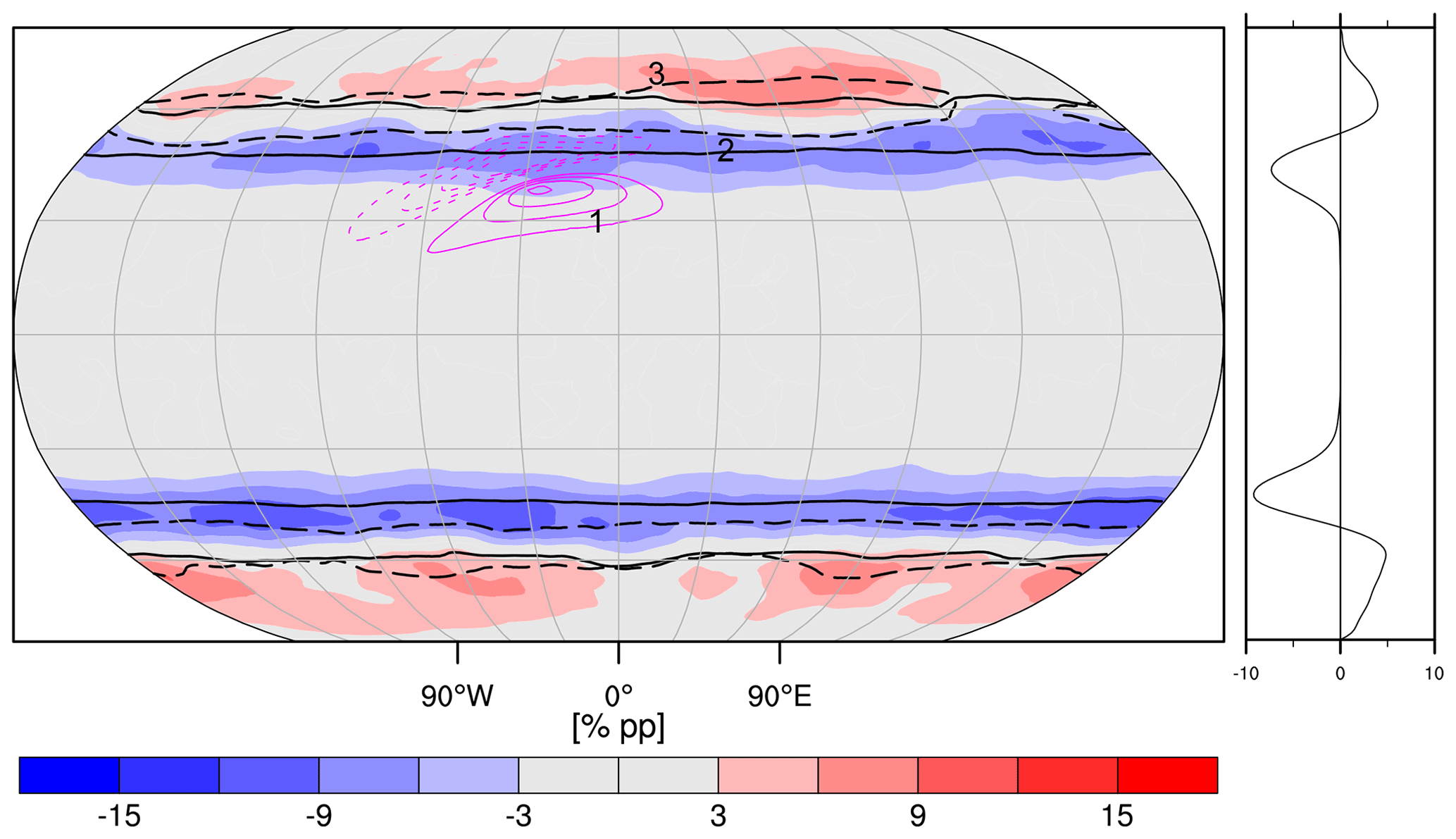
Figure 7 Change in surface cyclone frequencies (shading; percentage points) between warmed and control simulations. Additional black contours indicate absolute cyclone frequency of 20 % (dashed for the warmed simulation and solid for the control; as in the previous figures, the SST front is indicated by purple contours). Labels from Fig. 2 are superimposed.

Figure 7 shows the change in surface cyclone frequencies alongside the 20 % absolute cyclone frequency contour. Consistent with the changes in EAPE and EKE, high cyclone frequencies shift poleward in both hemispheres. In the zonal mean, the increase on the poleward side is spread over a wide band of latitudes, while the decrease on the equatorward side affects a smaller band of latitudes but reaches higher amplitude. Downstream of the SST front, the increase is confined to a region to the northeast of the front near 90–120^∘ E. Further downstream and far upstream, the frequency of cyclones decreases in the warmer simulation without being accompanied by an increase poleward of similar strength. These are regions that are also marked by a decrease in EAPE and external as well as internal baroclinic conversion in the warmed simulation, indicating an earlier termination of the intensified storm track. As shown below, this is in agreement with a reduced cyclone lifetime. Earlier termination of the storm track, accompanied by shortened cyclone lifetimes, is a feature observed under present-day climate conditions during mid-winter over the North Pacific, in particular for cyclones originating downstream of the Kuroshio SST front (Schemm et al., 2021). Earlier termination is also in agreement with an enhanced self-destruction mechanism (Kaspi and Schneider, 2011, 2013) that can be expected from the amplified stationary wave pattern (Fig. D1b).

4.2 Change in lifetime

The frequency distribution of the lifetimes of surface cyclones that have minimum lifetimes greater than 1 d is shown in Fig. 8a along with the median and 95th, 99th, and 99.9th percentiles on the lower axes (red dots correspond to percentiles in the warmer simulation, black dots to the control simulation). Lifetimes decrease in the warmer simulation for lifetimes greater than 3 d. While the median lifetime remains unchanged (red and black dots at 2.2 d), the lifetime tends to decrease for all percentiles greater than the 90th percentile (Fig. 8b).

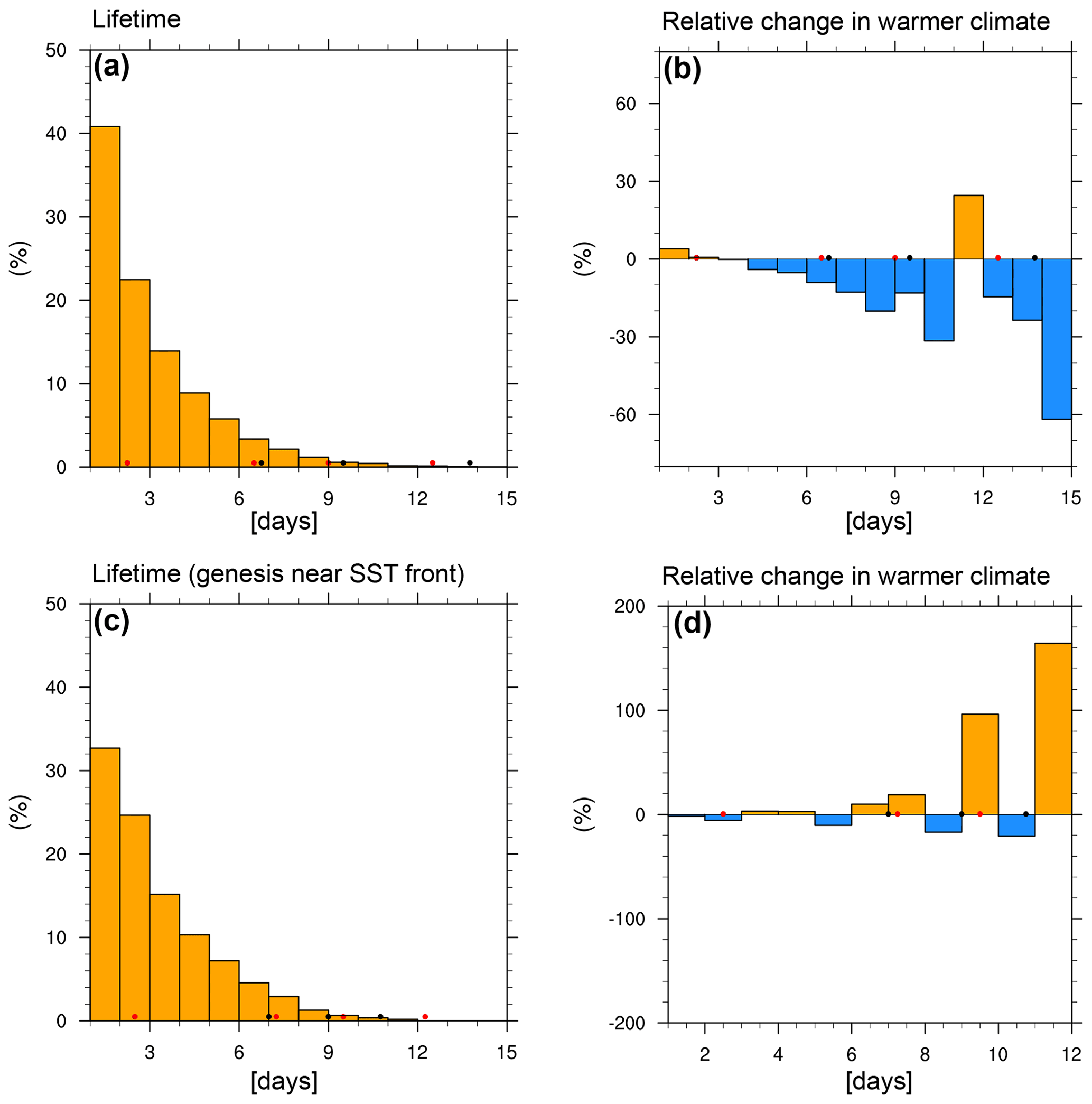
Figure 8 Frequency distribution of lifetimes of extratropical cyclones for (a) all cyclones (NH and SH) and (c) cyclones with genesis in the vicinity of the SST front in the control simulation. On the lower axes, dots indicate the median and the 95th, the 99th, and the 99.9th percentiles for the control (black) and +4 K (red) simulations. (b, d) Relative change of the distributions shown in (a) and (c) in the +4 K simulation. Note that the large relative change for the high percentiles results from the low number of cases in these bins. Note the different scaling in (b) and (d).

For cyclones originating near the SST front, the distribution of lifetimes is skewed towards longer lifetimes compared to all cyclones (Fig. 4c). While the lifetime of the median cyclone remains unchanged between the control simulation and the simulation with additional warming, the lifetime tends to increase for the high percentiles. For the 99.9th percentile, for example, it increases by more than 24 h. However, the upward trend alternates between bins and thus appears to be less robust compared to the general trend toward shorter lifetimes in the warmer simulation.

4.3 Change in deepening rates

The frequency distribution of cyclone deepening rates, calculated based on all 6 h minimum SLP changes along all cyclone tracks, has a median value of about 2 hPa (6 h)⁻¹ and is skewed towards larger deepening rates, with the 99th percentile in the control simulation at 10 hPa (6 h)⁻¹ (Fig. 9a). For cyclones originating near the SST front, the distribution of deepening rates is skewed toward even higher values; for example, the 99th percentile is 11 hPa (6 h)⁻¹ or higher by about half the median value (Fig. 9c). The frequency of very high deepening rates increases in the warmer simulation, while the frequency of deepening rates below the median of the control simulation decreases (Fig. 9b, d). Consequently, the high percentiles shift toward higher deepening rates; e.g., the 99th percentile decreases by about 1 hPa (6 h)⁻¹ for all cyclones and for those with genesis near the SST front, while the median changes only slightly.

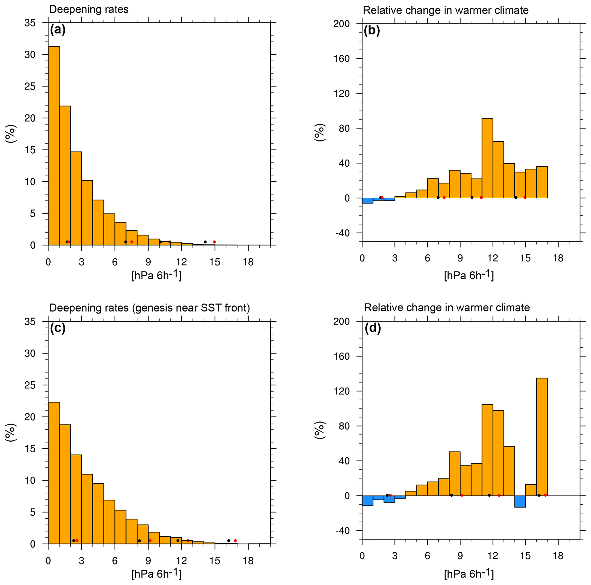
Figure 9 Frequency distribution of deepening rates, defined as 6-hourly minimum SLP changes, for (a) all cyclones and (c) cyclones with genesis in the vicinity of the SST front in the control simulation. On the lower axes, dots indicate the median and the 95th, the 99th, and the 99.9th percentiles for the control (black) and +4 K (red) simulations. (b, d) Relative change of the distributions shown in (a) and (c) in the +4 K simulation. Note that the large relative change for the high percentiles results from the low number of cases in these bins.

4.4 Change in maximum intensity

Maximum intensity is defined as the lowest SLP value found along a track, and based on each value from all tracks the frequency distribution in Fig. 10a is computed and for all tracks with genesis near the SST front in Fig. 10b. The distributions are normally distributed with median values in the control simulation approximately at 990 hPa and the 99th percentile found at 970 hPa (Fig. 10a, b). In the warmer simulation, the maximum intensity shifts towards lower pressure values. In particular for the very deep cyclones, the 99.9th percentile increases from 945 hPa to approximately 935 hPa (Fig. 10a). Overall, the median cyclone intensity in the control simulation becomes less frequent, while the frequency of very deep cyclones increases, and this increase is not limited to those cyclones with genesis near the SST front.

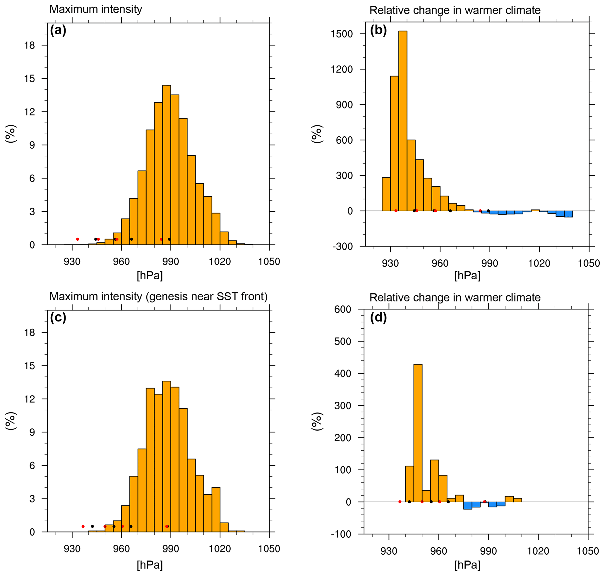
Figure 10 Frequency distribution of maximum intensity, defined as minimum SLP during the entire life cycle, for (a) all cyclones and (c) cyclones with genesis in the vicinity of the SST front in the control simulation. On the lower axes, dots indicate the median and the 95th, the 99th, and the 99.9th percentiles for the control (black) and +4 K (red) simulations. (b, d) Relative change of the distributions shown in (a) and (c) in the +4 K simulation.

4.5 Change in poleward propagation

In the following, we consider the poleward displacement of surface cyclones, which is defined as the meridional difference between genesis and lysis or genesis and the latitude of maximum intensity, respectively. The latter, in turn, is defined as the latitude at which the SLP minimum is observed along a track. The subsequent analysis is motivated by the reported enhanced poleward propagation of cyclones in a warmer climate (Tamarin and Kaspi, 2017; Tamarin-Brodsky and Kaspi, 2017). Poleward propagation of surface cyclones, which largely depends on a nonlinear mechanism, increases with the amplitude of lower- and upper-level disturbances (Gilet et al., 2009; Oruba et al., 2013). Consistently, the regions of high cyclone intensity are located where the strongest poleward motion occurs over the main ocean storm tracks (Besson et al., 2021). In a warmer climate, the increased moisture intensifies upper-level potential vorticity anomalies that more easily advect surface cyclones poleward (Coronel et al., 2015; Tamarin and Kaspi, 2016). Additionally, diabatic low-level potential vorticity (PV) generation eastward of the surface cyclone promotes intensification of the surface cyclone, and the interaction between the diabatically induced circulation and the cyclone also advects the cyclone poleward (Gilet et al., 2009; Coronel et al., 2015; Tamarin and Kaspi, 2016).

These earlier results suggest that cyclones with maximum deepening rates downstream of the SST front, which have been shown to be higher than elsewhere, exhibit advanced poleward displacement compared to cyclones elsewhere. The meridional displacement between cyclogenesis and cyclolysis, computed as the mean over all displacements, is 4.2^∘ latitude in the control run and 4.3^∘ latitude in the warmer run but under an on average reduced lifetime. A clearer picture emerges when considering only cyclones with maximum deepening rates downstream and in the vicinity of the SST front. The averaged displacement increases from 7.4^∘ latitude in the control simulation to 8.4^∘ latitude in the warmer simulation, in agreement with expectations. Here, it is in particular the poleward shift in lysis that dominates the change (56.5^∘ N in the control and 59^∘ N in the warmer simulations) because cyclogenesis is anchored near the SST front in both simulations. When the displacement is considered between cyclogenesis and maximum intensity, for all cyclones we find this to be on average 1.3^∘ latitude in the control run (downstream of the SST front 1.5^∘ latitude) and 1.0^∘ latitude in the warmer run (downstream of the SST front 1.1^∘ latitude). This appears at first to disagree with the results of Tamarin and Kaspi (2017) and Tamarin-Brodsky and Kaspi (2017). However, limiting the selection to the 200 deepest cyclones downstream of the SST front, which become even deeper in the warmer simulation and live longer, the poleward shift increases from 1.7^∘ latitude in the control simulation to 2.3^∘ latitude in the warmer simulation. Thus, while the majority of cyclones exhibit only marginal change in the poleward displacement until maximum intensity, the opposite is true for the strongest cyclones, which is also the selection criterion used by Tamarin and Kaspi (2017) and Tamarin-Brodsky and Kaspi (2017) and thus in agreement with these studies.

5 Conclusions

This study examines the response of the storm track downstream of an idealized SST front to uniform global warming by +4 K on an aquaplanet. The pattern of change reveals a tripole structure that has received little attention to date but is also seen in CMIP5 simulations under the RCP8.5 scenario when comparing present-day to end-of-century conditions over the North Atlantic and partly over the North Pacific. This tripole pattern consists of an EKE decrease upstream and equatorward of the front, an EKE increase downstream and northeast of the front, and a local reduction of EKE at polar latitudes just north of the SST front. Furthermore, the pattern is also evident in EAPE and the jet stream. The hemisphere without the SST front, in contrast, exhibits a rather zonally symmetric poleward shift.

A detailed analysis of the EAPE and EKE budgets shows that the tripolar change pattern in the first place is locally explained by increased or decreased external and internal baroclinic conversions, respectively, as well as changes to stationary waves in the case of the reduction of EAPE and EKE at polar latitudes. The SST front organizes the flow such that the baroclinic growth becomes more efficient downstream of the front; that is, the eddy heat flux better aligns with the baroclinicity vector. However, the hemisphere-wide change in baroclinic conversions is close to zero because it is reduced far downstream and upstream of the SST front compared to the control simulation. Notably, the SST front re-organizes and localizes baroclinic conversion without changing it globally and thus can be thought of as the chief organizer behind the spatial baroclinic conversion pattern. In the absence of a front, i.e., in the Southern Hemisphere in our simulations, the midlatitude meridional average of the changes of baroclinic conversions is thus also close to zero, indicating a poleward shift with little change in net conversion rates. Instead, the global increase in EAPE is explained by enhanced diabatic EAPE generation, primarily due to parameterized cloud physics and, in particular, resolved condensation. Diabatic EAPE tendencies due to longwave radiation are negative in the upper levels and positive in the lower levels and are partially offset by shortwave radiation. Turbulent generation of EAPE is partially offset by parameterized convection, especially near the SST front, with both changing sign over the front but in opposite directions.

Stationary waves further modify the EAPE and EKE patterns locally through advection. The amplitude of the stationary waves strengthens downstream and poleward of the SST front, most likely as a result of stronger eddy feedbacks (e.g., stronger diabatic heating and eddy heat/momentum fluxes in the warmer simulation). Upstream of the strengthened stationary trough in the warmer simulation, enhanced equatorward EAPE and EKE advection contributes to their local reduction at polar latitudes. Downstream between the strengthened stationary trough and the ridge, enhanced poleward EAPE and EKE advection leads to a local increase. The transition zone between the strengthened stationary trough and ridge also marks the end of the surface storm track. Hence, the self-destruction mechanism of storm tracks (Kaspi and Schneider, 2011, 2013) appears to be enhanced in the warmer simulation.

A feature-based surface cyclone detection scheme is used to detect changes in life cycle characteristics. Broadly consistent with previous idealized studies (Sinclair et al., 2020), we find a decrease in mean cyclone intensities and mean deepening rates, as well as an increase in strong cyclone intensities and strong deepening rates. This corresponds to a flatter probability density function of the two quantities in a warmer climate with a longer tail towards extremes. A reduction in mean lifetime is also noted, with the exception of the cyclones that form downstream of the SST front, which live longer in a warmer climate. The poleward displacement, defined as the latitudinal shift between genesis and lysis, remains fairly unchanged when averaged over all cyclones but increases for cyclones with genesis downstream of the SST front. Defined as the latitudinal shift between genesis and location of maximum intensity, instead of lysis, the poleward shift even decreases when averaged over all cyclones but increases for the subset of the 200 strongest cyclones, which is consistent with Tamarin and Kaspi (2017). Again, the probability density function becomes flatter with longer tail. The most notable difference between all cyclones and those with genesis at the SST front is the opposite response of their lifetimes to warming. Finally, it is noted that the number of cyclones decreases by about 15 %.

Limitations and future direction

The main limitation of this study is its idealized nature. The ocean acts as infinite source and sink of heat, which is not balanced by ocean heat uptake elsewhere. A slab ocean would be a useful extension to our setup. Consideration is given in this study to the main EAPE and EKE source and sink terms, but a study on the redistribution of EAPE and EKE by changes in advection and ageostrophic flux around the SST front (Orlanski and Katzfey, 1991) would be interesting to further elucidate the changes in the internal structures of the storm track such as the downstream development.

It should be noted that the zonal asymmetry created by the rotated SST anomalies unlikely reflects the influence of the Gulf Stream front alone but rather the combined land–sea contrast including the Gulf Stream SST front. The lack of an upstream mountain range and an interactive ocean could be one reason for the different magnitude of EKE change in our idealized model compared to the CMIP models.

Future studies may also probe the sensitivity of the formation of the EKE tripole pattern to the shape, strength, and orientation of the imposed idealized SST front and to the used model resolution. A detailed analysis of the sensitivity of the baroclinic conversions, its efficiency, and the vertical tilt of eddies at the SST front, as well as the sensitivity to the specifics of the SST front (shape, orientation and strength) is left for future research. Further studies may also consider changes in special cyclone types, such as frontal-wave cyclones (Schemm and Sprenger, 2015) or diabatic Rossby waves (Boettcher and Wernli, 2013).

Appendix A: Initial SST profile

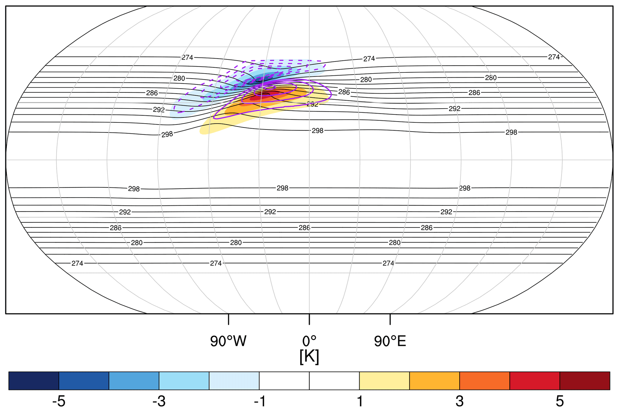
Figure A1 Zonally symmetric initial SST profile known as “Qobs” (black contours), additional SST anomaly used to construct the SST front (colored shading), and resulting 2 m temperature anomaly calculated as a deviation from the climatological zonal mean 2 m temperature (purple contours with solid lines indicating positive values and dashed lines negative values; ±1, 1.5, 2, and 2.5^∘). The latter is shown in all figures in the paper.

Appendix B: Zonal mean change

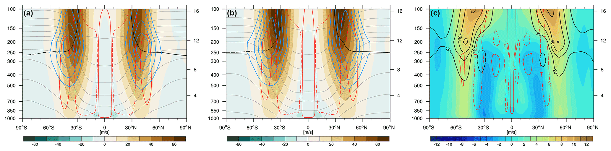
Figure B1 Zonal mean fields in the (a) control and (b) control +4 K simulations and (c) their difference for the zonal wind speed (shading; m s ⁻¹), vertical wind speed (red contours, negative dashed; cm s ⁻¹), and eddy kinetic energy (blue contours in a and b and black contours in c​​​​​​​; J kg,⁻¹). Additionally shown in (a) and (b) is the dynamical tropopause (black contour; 2 PVU) and potential temperature (gray contours).

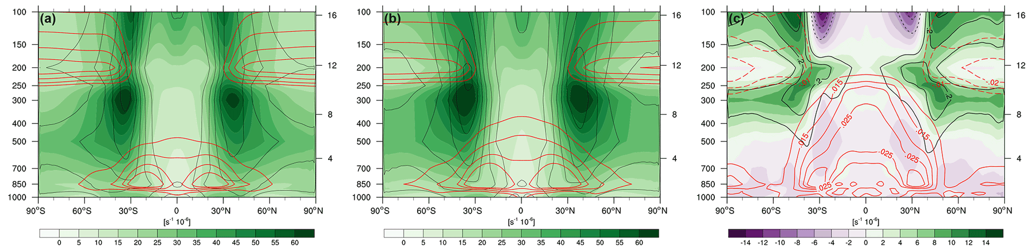
Figure B2 Zonal mean baroclinicity (green shading; s ⁻¹ × 10⁻⁶), meridional potential temperature gradient (black contours; K (100 km)⁻¹), and the dry static stability normalized by the scale height (red contours; K² m⁻² s²) in the (a) control and (b) control +4 K simulations and (c) their difference.

Appendix C: Individual diabatic EAPE tendencies in the control simulation

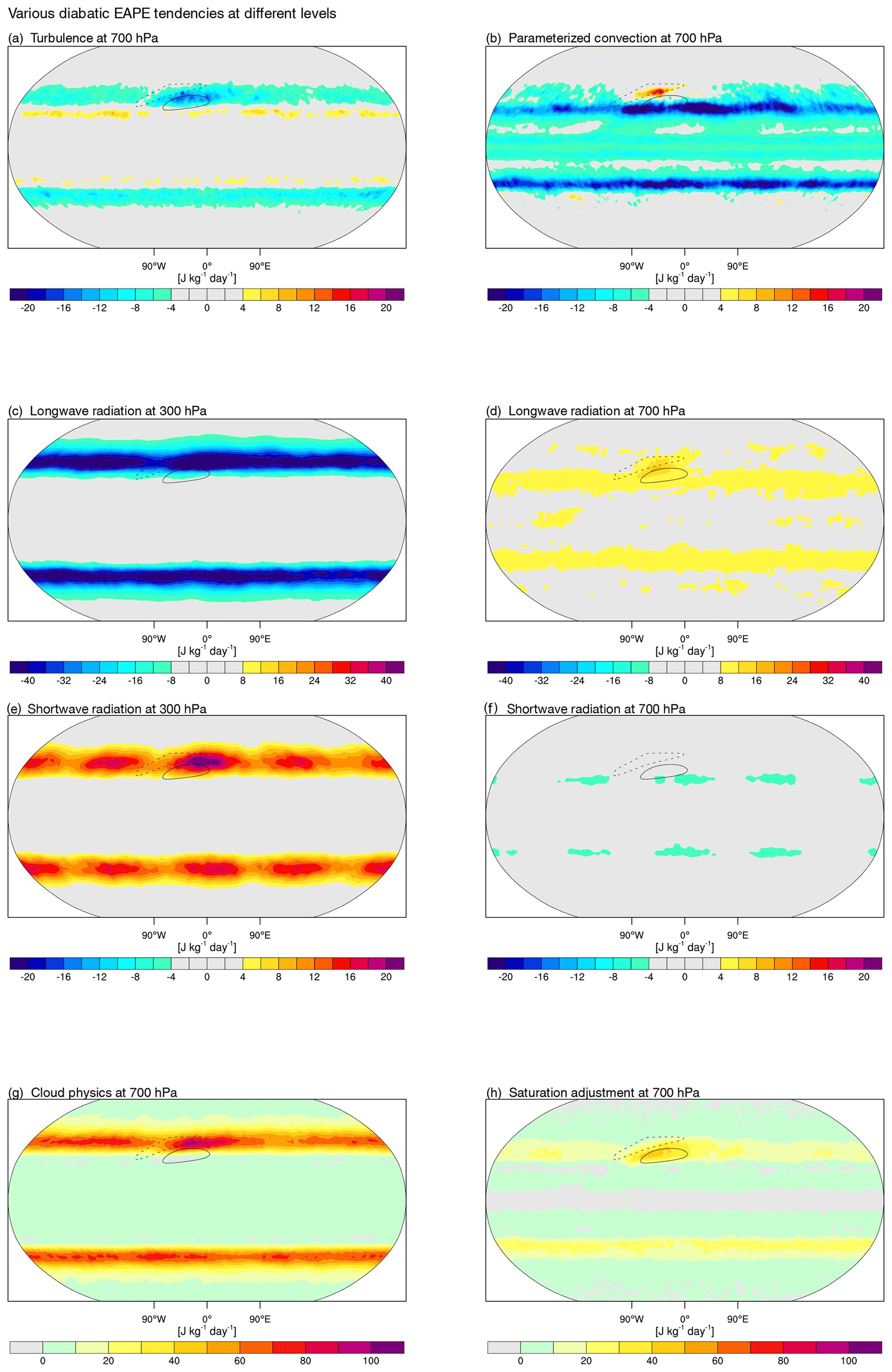
Figure C1 Diabatic EAPE tendencies for different processes on different selected levels for the control simulation. Note the different scaling for each panel. EAPE tendencies due to (a) turbulence and (b) parameterized convection at 700 hPa, longwave radiation at (c) 300 and (d) 700 hPa, shortwave radiation (e) at 300 and (f) 700 hPa (note reduced scaling by a factor of 2 compared to longwave radiation), (g) cloud physics, and (h) saturation adjustment at 700 hPa. Units are J kg⁻¹​​​​​​​ d⁻¹.

Appendix D: Response of the jet stream and stationary waves

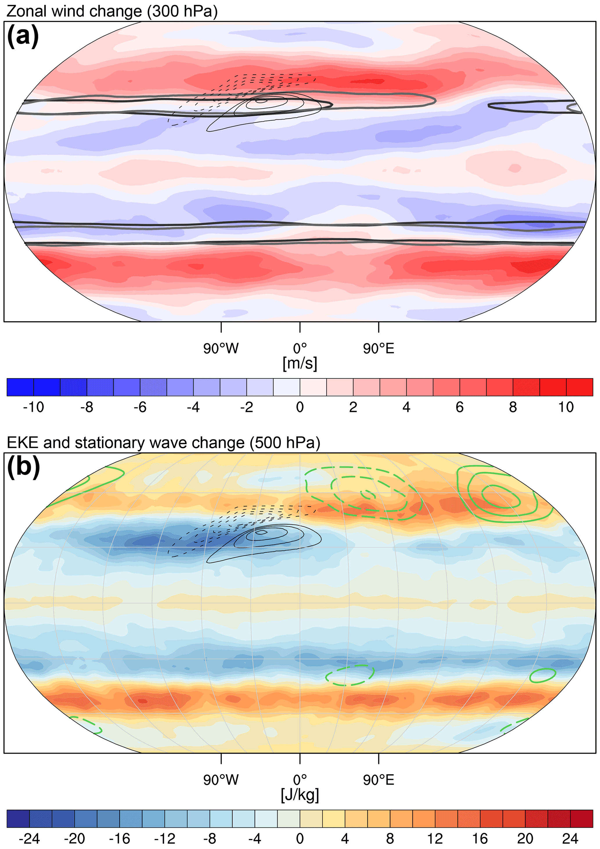
Figure D1 (a) Wind speed difference at 300 hPa between the Qobs control run with SST front in the Northern Hemisphere and uniform warming by 4 K at the surface, as well as the 40 m s⁻¹ wind speed contour in the control (black) and the warmed simulations (gray). (b) EKE (color) and geopotential difference at 500 hPa (defined as deviation from the zonal mean; green solid indicate positive and dashed negative values; ±200, 400, and 600 m² s⁻²). Additionally shown in both panels is the 2 m temperature after removing the zonal mean (black solid contours indicate positive and dashed negative values; starting at ±2.5 K in steps of 0.5 K).