Assessing the plausibility of unprecedented events: a process-based approach applied to month-long heatwaves in Western Europe

Climate model based storylines of individual climate and weather events are increasingly used to quantify impacts, vulnerability, or stress-test infrastructure to inform adaptation decisions. Here, we present an approach to test the plausibility of unprecedented climate storylines based on physical conformity, internal consistency, and historical precedent. We apply this approach to assess the plausibility of month-long heatwaves in Western Europe that would exceed existing record temperatures by more than 5 K. These heatwaves are based on model simulations using ensemble boosting, a computationally efficient method to simulate unprecedented events. We compare these unprecedented heatwaves with historical heatwaves in a reanalysis data set, using standardised anomalies relative to a time-evolving climatology of relevant physical variables. We show that these unprecedented heatwaves are associated with well-known physical drivers that are similar to historical heatwaves, including strong anticyclones and low soil moisture. The anomalies of these drivers are more intense in magnitude, but similar in their spatial patterns and in their relationships with each other. However, we also reveal substantial discrepancies between historical and unprecedented heatwaves, which are related to atmospheric blocking, land-atmosphere interactions, and their temporal persistence. Despite these discrepancies, we conclude that these long-lasting, unprecedented heatwaves should not be ruled out as implausible and thus highlight the need to anticipate such events when planning adaptation measures. Similar approaches can be used to assess the plausibility of other types of extreme events.

1 Introduction

Unprecedented events represent a particularly difficult challenge for extreme event research: It is essential to study them for disaster preparedness, but their absence from reanalysis records limits our ability to make robust statements about their potential magnitude and characteristics (Fischbacher-Smith, 2010; Kelder et al., 2025). Unprecedented events can be simulated in climate models, but the lack of comparable historical analogues leads to the fundamental question whether these simulated events are plausible to occur in the real world. The importance of anticipating future unprecedented events has been further highlighted by recent extreme events such as the 2021 Pacific North West heatwave, which broke previous temperature records by almost 5 K (Bartusek et al., 2022; White et al., 2023; Fleishman et al., 2025). Here we assess the plausibility of simulated month-long heatwaves in Western Europe that would exceed existing records by similar margins (Lüthi et al., 2024).

Future record-breaking events can be studied using climate storylines, which provide physically self-consistent unfoldings of plausible future events, making it possible to study their characteristics and underlying physical processes (Hazeleger et al., 2015; Shepherd et al., 2018; Sillmann et al., 2021; Baulenas et al., 2023; van den Hurk et al., 2023; Baldissera Pacchetti et al., 2024). Among other approaches, such unfoldings can be selected from single-model initial-condition large ensembles of climate models (Bador et al., 2017; van der Wiel et al., 2021; Suarez-Gutierrez et al., 2020; Fischer et al., 2021) or from ensembles of weather prediction models (UNSEEN approach, van den Brink et al., 2005; Thompson et al., 2017). Furthermore, model ensembles can be optimised to simulate more frequent and intense extreme events by using rare event algorithms such as the GKTL algorithm (Giardina et al., 2011; Ragone et al., 2018; Ragone and Bouchet, 2021; Yiou et al., 2023; Noyelle et al., 2025a, b), ensemble boosting (Gessner et al., 2021; Fischer et al., 2023; Lüthi et al., 2024; Suarez-Gutierrez et al., 2025), or based on adaptive multilevel splitting (Finkel and O’Gorman, 2024, 2026). In recent years, similar approaches have been used to create extreme event storylines using machine learning (Mahesh et al., 2025a, b; Whittaker and Di Luca, 2026). However, how can we test whether simulated unprecedented events are plausible to occur in the real world?

Assessing the plausibility of unprecedented events is essential because it informs us about the potential intensity of events that society needs to prepare for (Nordmann, 2013). This makes plausibility an essential criterion for decision making, such as for natural disaster preparations (van der Helm, 2006; Shepherd et al., 2018; Sillmann et al., 2021) and is useful in a wide range of fields, ranging from epidemiology to economics (Derbyshire, 2022; Goodwin and Wright, 2010). This is because studying extreme events that are considered plausible – irrespective of their probability of occurrence – allows for the exploration of future scenarios while embracing inherent uncertainties (Selin and Guimarães Pereira, 2013). Therefore, studying plausible future extremes is essential for providing tangible what-if scenarios that are needed to inform disaster preparation.

But what does plausible mean? Located between possible (without contradiction) and probable (likely to occur), plausible is associated with being credible, trustworthy, and reasonable (Amara, 1991; Wilson, 1998; Selin, 2006; van der Helm, 2006; Nordmann, 2013; Urueña, 2019). However, the concept of plausibility is based on subjective judgement, and thus there are no universal criteria (Selin and Guimarães Pereira, 2013). In this work, we base our assessment of plausibility on tangible criteria suitable for climate storylines: conformity with physical principles, internal consistency, and historical precedent (Amara, 1991; Nordmann, 2013; Shepherd et al., 2018). These criteria can be used to either affirm or question the plausibility, depending on whether the underlying physical processes are internally consistent with process understanding and externally supported by historical events. Fundamentally, it is not possible to conclusively prove that a given event is plausible; the only feasible approach is to perform a series of tests in which the confidence increases with the number of distinct tests performed.

There are a number of different ways to translate plausibility criteria into concrete analysis steps. Most commonly, the plausibility of simulated extremes is statistically analysed through extreme value theory and model fidelity tests, for example, by comparing statistical distributions and moments of model output with observations or reanalysis (Thompson et al., 2017, 2019; Vautard et al., 2019; Philip et al., 2020; Kelder et al., 2022a, b). In contrast, only few studies assess the plausibility of simulated extreme events by analysing the physical processes that drive them, for example, by studying the temporal evolution of variables and the correlations between them (Vautard et al., 2019; Kelder et al., 2022b) or the dynamic and thermodynamic precursors of the events (Klif et al., 2026). An important part of this assessment involves comparisons with historical events; however, there are inherent limitations of this approach when analysing unprecedented extremes in a transient climate. This is particularly obvious for extreme events that are directly affected by global and regional warming trends; for example, heatwaves that reach previously impossible temperatures are becoming possible in a warming climate (Fischer et al., 2025). To account for this, we propose a process-based approach centred around standardised anomalies with respect to a time-evolving climatology, that is, we quantify how extreme an event is relative to the background climate (mean and variability) in which it occurs. This allows us to directly and systematically compare anomalies in a wide range of physical drivers during simulated unprecedented events with anomalies during historical events and to evaluate their consistency with current process understanding. In this way, we expand on existing process-based studies and offer an additional layer of evidence to complement statistical approaches.

To demonstrate our approach, we focus on heatwaves in Western Europe. This is motivated by the fact that both mean summer temperatures and extreme heat in Western Europe are increasing faster than in almost any other region, caused by a combination of anthropogenic global warming, regional reductions in aerosol emissions, and changes in circulation (Singh et al., 2023; Vautard et al., 2023; Schumacher et al., 2024; World Meteorological Organization et al., 2025). As a consequence, Western Europe has been a hotspot for record-breaking heat extremes: Since the turn of the 21st century, Western Europe experienced record-breaking heat extremes in 2003, 2006, 2015, 2018, 2019, 2022, 2025, and most recently in 2026 (Rebetez et al., 2009; García-Herrera et al., 2010; Russo et al., 2015; Kornhuber et al., 2019; Sánchez-Benítez et al., 2022; Feser et al., 2024; Hotz et al., 2024; Copernicus Climate Change Service, 2025; World Meteorological Organization, 2026). Given current global warming trends, the likelihood of record-breaking heatwaves is expected to increase further in the future (Fischer et al., 2025), with parts of Western and Central Europe among the most at-risk regions for such heatwaves (Thompson et al., 2023).

The processes that govern heatwaves occur on a wide range of spatial and temporal scales and include interactions between the atmosphere, ocean, cryosphere, land surface, and biosphere (Barriopedro et al., 2023; Domeisen et al., 2023). In mid-latitudes, heatwaves are often caused by quasi-stationary Rossby wave packets that lead to persistent anticyclones (Röthlisberger et al., 2019). These anticyclones can disrupt the zonal atmospheric circulation leading to atmospheric blocking (Drouard and Woollings, 2018; Röthlisberger and Martius, 2019; Kautz et al., 2022). In summer, this can favour heat extremes through horizontal temperature advection, vertical adiabatic subsidence, and diabatic heating at the surface through solar radiation and turbulent fluxes (Zschenderlein et al., 2019; Barriopedro et al., 2023; Röthlisberger et al., 2026). These surface fluxes are often amplified by land-atmosphere feedbacks (Fischer et al., 2007; Seneviratne et al., 2010), particularly during persistent heatwaves that last multiple weeks (Tuel and Martius, 2023; Pappert et al., 2025). These generally well-understood physical drivers provide the foundation for our process-based approach to assess plausibility.

Heatwaves have severe impacts on human health, ecosystems, and infrastructure (Easterling et al., 2000; Zuo et al., 2015), and these impacts can be particularly severe during long-lasting heatwaves (D'Ippoliti et al., 2010; Anderson and Bell, 2011; Polt et al., 2023). Prominent examples of long-lasting heatwaves include the Eastern European heatwave of 2010 (Barriopedro et al., 2011; Dole et al., 2011) as well as the Western European heatwaves of 1976 (Green, 1977; Kendon et al., 2024) and 2003 (Black et al., 2004; García-Herrera et al., 2010), which resulted in thousands of excess deaths (Le Tertre et al., 2006; Robine et al., 2007). Recent model experiments based on ensemble boosting suggest that persistent, month-long heatwaves that would break reanalysis records by more than 5 K in Western Europe are possible in the near future, which would have severe effects on heat-related mortality (Lüthi et al., 2024). Given the unprecedented nature of these month-long heat extremes, here we address the pressing question whether they are plausible to occur in the real world.

2 Methods

2.1 Climate model and reanalysis data

We create unprecedented heatwave storylines using ensemble boosting simulations in CESM2 with daily model output (see Appendix A). As a climatological reference, we use daily output of the 100-member CESM2 large ensemble (LE) that follows the historical (1850–2014) and SSP3-7.0 (2015–2100) scenarios (Danabasoglu et al., 2020; Rodgers et al., 2021). Most of the atmospheric and surface variables that we use are available as model output (Table C). Exceptions are the diurnal temperature range (DTR, the difference between daily maximum temperature TX and daily minimum temperature TN), total precipitation (PREC, the sum of convective and large-scale precipitation), and the evaporative fraction (EF, calculated from the surface fluxes of latent heat LHF and sensible heat SHF as $\text{EF}=\text{LHF}/(\text{LHF}+\text{SHF})$).

To compare with historical heatwaves, we use daily output of the ERA5 reanalysis for 1950–2025 (Hersbach et al., 2020) for all variables in Appendix C except for SM, for which we use ERA5-Land instead (Muñoz-Sabater et al., 2021). In addition to these quality-checked final products, we use preliminary ERA5 and ERA5-Land data for the month-long heatwave in Western Europe from 17 June to 16 July 2026 (Hersbach et al., 2020; World Meteorological Organization, 2026).

For the temperature budget analysis, we additionally use daily model output on the 850 hPa level from the boosting simulations and from ERA5 for the temperature (T850), zonal wind (U850), meridional wind (V850), and vertical wind (ω850), as well as the temperature tendency due to physical parametrisations. In CESM2, this is available as the PTTEND variable, in ERA5 we use the avg_ttpm variable which is only available from the deterministic forecast model.

For SM, the top-layer of the soil differs between CLM, CESM2's land model (top 10 cm) and ERA5-Land (top 7 cm). To compare the absolute values of SM, the ERA5 values (volumetric soil water in m³ m⁻³) are converted to CESM2 units (soil water mass in kg m⁻²). Performing the same analysis for the top 1 m of the soil does not alter our conclusions (not shown).

We focus on a box in Western Europe (WE) where the boosting simulations detect heatwaves that exceed historical records by particularly large margins (0–10° E, 46–51° N). All CESM2 and ERA5 variables are averaged over this domain before we calculate standardised anomalies (see below). To study large-scale conditions, we further use the full horizontal fields of all variables analysed in Europe (12° W–42° E, 35–72° N). For this analysis, we remap the horizontal ERA5 fields to the CESM2 grid using first order conservative remapping (Schulzweida, 2023). Unless stated otherwise, all of our analysis is performed for the summer months of June, July, and August (JJA).

2.2 Standardised anomalies

To enable a meaningful comparison between the unprecedented heatwave storylines and historical heatwaves, we express every variable x as standardised anomaly z_x (in the following simply “anomaly”):

$$\begin{array}{}\text{(1)}& z_x(r,y,s)={\displaystyle \frac{x(r,y,s)-\stackrel{\mathrm{‾}}{x}(r,y\pm \mathrm{15}\mathrm{years},s\pm \mathrm{2}\mathrm{d})}{x^{\prime }(r,y\pm \mathrm{15}\mathrm{years},s\pm \mathrm{2}\mathrm{d})}}.\end{array}$$

Here, the region r refers to an individual grid cell of the CESM2 grid or the box-average over WE, y refers to the year, s refers to the day of the summer season (JJA), and $\stackrel{\mathrm{‾}}{x}$ and x^′ refer to the mean and standard deviation of x, respectively, calculated over a centred 31-year window in time and a centred 5 d window over the seasonal cycle.

For the boosting simulations, $\stackrel{\mathrm{‾}}{x}$ and x^′ are derived using the full 100-member CESM2-LE, except for SM, which is available for only 90 members. For CESM2-LE itself, the standardisation is performed for the period 2005–2035 (the same period as the 35-member CESM2 ensemble on which the boosting simulations are based). For ERA5, the standardisation is limited to the period 1965–2010, where a centred 31-year reference period can be constructed based on the data record available at the time of the analysis. When LHF and SHF are of opposite sign but similar magnitude, this can lead to very large absolute values in EF locally, particularly over ocean. Thus, only grid cells with $\mathrm{0}<\text{EF}<\mathrm{1}$ are used to calculate EF anomalies.

The standardisation is performed separately for daily values and a 30 d running mean. The 30 d running mean is assigned to the “central day”, the 15th day within a given 30 d period. We consider all 30 d periods whose central day lies in JJA, including periods that start in May or end in September. To calculate the 30 d running mean of the box-mean over WE, we require data points on all 30 d within a given window; for the running mean of individual grid points, this is relaxed to at least 25 data points within a 30 d window in order to reduce the effect of individual missing values in EF (see above).

2.3 Heatwave selection

Based on anomalies in the 30 d running mean of TM in WE, we select all 20 heatwaves in our boosting simulations that exceed the most extreme heatwave in ERA5 (“unprecedented” heatwaves U1–U20, Table B1). From ERA5, we select all 30 d periods whose TM anomalies in WE exceed the 95th percentile of all JJA 30 d means in the reanalysis record, yielding a total of 11 “historical” heatwaves (Table B2). Our anomaly-based approach limits the reanalysis record to 1965–2010, which excludes many of the most extreme heatwaves that occurred in the last 15 years. Thus, we also perform the same analysis for the absolute TM values in WE in 2011–2026, which yields 10 “recent” historical 30 d heatwaves (in 2013, 2015, 2018, 2019, 2020, 2022, 2023, 2024, 2025, and 2026).

To avoid selecting temporally overlapping heatwaves, we only consider the largest 30 d anomaly of each boosting run, and only consider the largest 30 d anomalies within ±30 d in ERA5, allowing more than one heatwave per year to be selected. In this way, we select the 30 d periods that feature the most anomalously high temperatures with respect to the background climate and the timing within the summer season in which they occur. To directly compare the historical heatwaves to CESM2 heatwaves of similar magnitude, we select the 20 heatwaves in CESM2-LE with the most similar 30 d TM anomaly over WE for each historical heatwave, separately for two different periods (the historical period 1965–2010 and the period of the boosting simulations 2005–2035). In total, we thus select 220 “moderate” CESM2 heatwaves for each climate period, whose TM anomalies differ from the respective historical heatwave by at most ±0.1 σ (Fig. 1a).

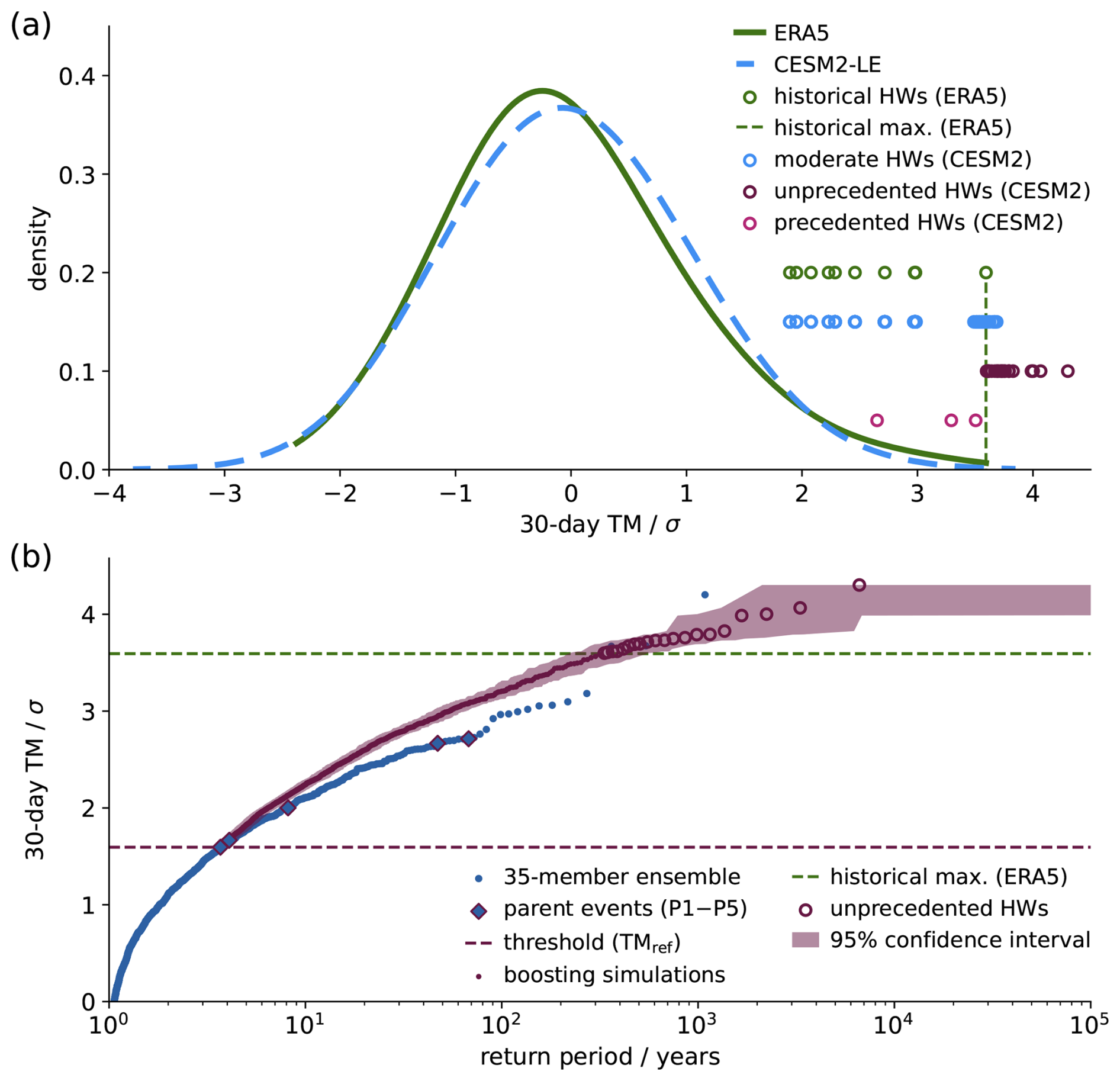
Figure 1 Unprecedented month-long heatwave storylines in Western Europe. (a) 30 d TM anomalies of the most extreme historical heatwaves (green circles), moderate heatwaves in CESM2-LE with the same TM anomalies (light blue circles), precedented (pink circles) and unprecedented heatwaves (purple circles) from ensemble boosting. Kernel density estimates of 30 d TM anomalies during JJA in ERA5 (1965–2010, green line) and CESM2-LE (2005–2035, light blue line), using a Gaussian kernel with a bandwidth of 0.5 σ, truncated at the data limits. (b) Return period estimates of 30 d TM anomalies from boosting simulations (purple dots), including the selected unprecedented heatwaves (purple circles), and their 95 % confidence interval, as well as return period estimates of heatwaves in 35-member CESM2 ensemble (dark blue dots), including the selected parent heatwaves (dark blue diamonds). The thresholds for the return period calculation (TM_ref, dashed purple) and for the selection as unprecedented heatwave (historical maximum, dashed green) are also shown.

Of the 20 unprecedented heatwaves in our simulations, 15 originate from the same parent ensemble P1 (model year 2015), and the other five come from a second parent ensemble P2 (model year 2031). Unprecedented heatwaves from the same parent feature quite similar SM anomalies, but are still distinct in their atmospheric conditions (Fig. B1) and in the relative importance of relevant physical drivers (Fig. B2b). Nevertheless, to increase the independence and representativeness of the analysed heatwaves, we also include in our analysis the most extreme 30 d heatwaves of the three other parent ensembles P3–P5 (model years 2030, 2028, and 2028). However, because their 30 d TM anomalies are smaller than the most extreme historical heatwave, they are not considered “unprecedented” heatwaves and instead analysed separately.

2.4 Temperature budget analysis

Following Tyrlis et al. (2013) and Garfinkel et al. (2024), the Eulerian temperature budget can be written as

$$\begin{array}{}\text{(2)}& \underset{\text{local}}{\underbrace{{\displaystyle \frac{\partial T}{\partial t}}}}=\underset{\text{zonal}}{\underbrace{-{\displaystyle \frac{u}{r\cos \left(\mathit{\varphi }\right)}}{\displaystyle \frac{\partial T}{\partial \mathit{\lambda }}}}}\underset{\text{meridional}}{\underbrace{-{\displaystyle \frac{v}{r}}{\displaystyle \frac{\partial T}{\partial \mathit{\varphi }}}}}\underset{\text{adiabatic}}{\underbrace{-{\displaystyle \frac{T}{\mathit{\theta }}}{\displaystyle \frac{\partial \mathit{\theta }}{\partial p}}\mathit{\omega }}}\underset{\text{diabatic}}{\underbrace{+{\displaystyle \frac{J}{C_p}}}}+\text{residual},\end{array}$$

where T is the temperature, t is the time, u, v, and ω are the zonal, meridional, and vertical wind components, θ is the potential temperature, p is pressure, ϕ is latitude, λ is longitude, r is the radius of Earth, J is the diabatic heating rate, and C_p is the heat capacity of air at constant p. In this way, the local temperature tendency is decomposed into four terms: zonal temperature advection, meridional temperature advection, adiabatic changes resulting from vertical temperature advection, and diabatic sources and sinks (such as radiation, evaporation/condensation, and surface exchanges), as well as a residual term.

For historical and recent heatwaves in ERA5 (except 2026), and for precedented and unprecedented heatwaves in CESM2, we evaluate Eq. (2). To reduce the effects of topography, we focus on the 850 hPa level (Tyrlis et al., 2013; Garfinkel et al., 2024). We calculate the zonal, meridional, and adiabatic terms from second order centred differences of daily model output on the native grids of ERA5 and CESM2, but the results are not sensitive to spatial remapping. For the diabatic term, we use the daily mean temperature tendency due to physical parametrisations. The resulting values are averaged over WE, and separately averaged over days with positive and negative local T tendencies during each event.

2.5 Persistence

To analyse temporal persistence, we calculate the number of consecutive days on which daily anomalies are $\ge +\mathrm{1}\mathit{\sigma }$ (for TM and Z500) or $\le -\mathrm{1}\mathit{\sigma }$ (for SM). For ERA5 and CESM2-LE, we count the occurrences of consecutive days whose end date lies in JJA and divide this count by 92 to yield the frequency per summer season. For precedented and unprecedented heatwaves, we use the longest persistence duration that ends in the respective boosting run, including periods that start in the parent run. Thus, persistence durations from all sources can include days in months preceding JJA.

We analogously evaluate the persistence of atmospheric blocking using a simple blocking index (Tibaldi and Molteni, 1990), setting the northern and southern latitudes to the edges of our European domain (35–72° N). A day counts as blocked, if Z500 satisfies both blocking criteria of Tibaldi and Molteni (1990) for at least one longitude within our WE domain (0–10° E). All calculations are performed on the CESM2 grid, but spatial mapping has only a negligible effect.

2.6 Multilinear model

We construct a multilinear statistical model based on a multivariate ordinary least-squares regression. For simplicity, we focus on a set of five predictors (Z500, U500, V500, SM, SSR) and apply it separately for three different prognostic variables (TM, TX, and TN). For each prognostic variable, the model is fitted to the maxima of 30 d z_TM of each summer season, with separate versions trained on ERA5 and CESM2-LE. This gives six different model versions which we use to infer anomalies in the prognostic variable during the unprecedented heatwaves based on the simulated anomalies of the five predictors as

$$\begin{array}{}\text{(3)}& z_{x,\text{inf}}\left(d\right)=\sum _p{\mathit{\beta }}_p{z}_p.\end{array}$$

Here, $x\in [\text{TM},\text{TX},\text{TN}]$ is the prognostic variable, $p\in [\text{Z500},\text{U500},\text{V500},\text{SM},\text{SSR}]$ are the predictors, $d\in [\text{CESM2-LE},\text{ERA5}]$ are the data sources on which the model is trained, and β_p are the coefficients of the model.

The predictors were chosen as a compromise between the simplicity of the model and the inclusion of the most important processes that govern the unprecedented heatwaves. Z500 is chosen due to the importance of anticyclones for mid-latitude heatwaves. Because our model is based on WE-mean anomalies, it does not contain any information on the position of the anticyclone relative to WE, for which we include U500 and V500 as predictors. SM is included to capture the important role of low soil moisture during heatwaves, and SSR is included to account for the diabatic contribution of radiation.

The model is meant to be a simplified representation of the relevant physical processes that drive month-long temperature extremes in Western Europe. Inherently, it cannot capture processes involving variables not included in the model, or non-linear relationships, including, but not limited to, land-atmosphere feedbacks between soil moisture and temperature. To further investigate this, we employ a modified version of the model to infer anomalies in SHF, LHF, and EF. As predictors, we chose TM, SM and SSR, which are the variables most directly linked to the variables inferred in the absence of atmospheric humidity or near-surface wind in our analysis set of variables.

3 Results

To evaluate plausibility, we focus on storylines of unprecedented month-long heatwaves, defined as periods during which the 30 d running mean TM anomaly in WE surpasses the most extreme historical heatwave in June/July 1976 (3.6 σ, the only historical event exceeding 3 σ, see Table B2). In our CESM2 boosting simulations, we identify 20 such unprecedented heatwaves (labelled U1–U20), with anomalies between 3.6 σ and 4.3 σ (purple circles in Fig. 1a, Table B1, Sect. 2.3). The return period estimates of these unprecedented heatwaves range from around 300 years to more than 6000 years, with 95 % confidence intervals of 200–2000 years (lower bounds) to 500 years–∞ (upper bounds), with infinite upper bounds for the three most extreme heatwaves (Fig. 1b; see Appendix A). By centring our assessment on the most extreme heatwaves in our simulations, we target the events that are most likely to be influenced by limitations in the applicability of CESM2. However, this approach also comes with some drawbacks. In addition to the limited sample size of unprecedented heatwaves in our simulations (n=20), they originate from only two different parent ensembles, leading to similar preconditions in slow components such as the land surface (Sect. 2.3, Fig. B1c).

We address this challenge in two ways: (1) We increase the representativeness of our analysis by additionally including the most extreme heatwaves of the three other parent ensembles in our simulations for some of our assessments. Because their anomalies are smaller than the most extreme historical heatwave, we refer to them as “precedented” heatwaves (Sect. 2.3, pink circles in Fig. 1). (2) Using large-deviation theory, it has been shown that the typicality of heatwaves tends to increase with their magnitude, that is, more extreme heatwaves tend to become more similar in their physical pathways, as they require a “perfect storm” of strong contributions by most relevant heatwave drivers to occur (Lucarini et al., 2023; Noyelle et al., 2024). For this reason, we expect many of our findings to also apply to other unprecedented heatwaves as well as to less extreme heatwaves that might only exhibit a subset of these heatwave drivers. Furthermore, if even the most extreme heatwaves simulated by CESM2 are considered plausible, this ultimate test also improves confidence in CESM2 to simulate less extreme heatwaves.

Given that the central return period estimates for the unprecedented heatwaves analysed here are finite but much longer than a human lifetime, they appear statistically possible but not probable. In the following, we address the less straight-forward question of whether these unprecedented heatwaves are plausible by assessing their physical conformity, internal consistency, and historical precedent. In practice, our assessments of these characterisations naturally overlap, but generally fall into two categories: (1) By comparing the unprecedented heatwaves from CESM2 ensemble boosting simulations to less extreme heatwaves in CESM2-LE, we assess their internal consistency within the CESM2 model. This allows us to test whether the processes present during these unprecedented heatwaves are similar to those simulated during less extreme heatwaves in CESM2. (2) By comparing them to historical heatwaves, we assess whether – despite their by definition unprecedented magnitude – these heatwaves have external empirical support from historical precedents. This allows us to test whether the processes present during these unprecedented heatwaves are similar to heatwaves in the reanalysis record.

The conformity to physical principles represents the foundation of most of our assessment procedure; we test it by comparing the underlying physical processes in these unprecedented heatwaves both internally (within CESM2) and externally (with ERA5). In this way, we test the ability of CESM2 to realistically simulate extreme heatwaves with intensities beyond those found in the reanalysis record. The overall result of our assessment – whether the evidence supports or questions plausibility – depends on the combined results of several analysis criteria, which we present in the following.

3.1 Spatial fields

We start by exploring the large-scale spatial behaviour of unprecedented heatwaves over Europe. For this, we compare the composite spatial fields of 30 d anomalies during unprecedented and historical heatwaves for relevant heatwave variables (Fig. 2). In this context, it would support plausibility if TM anomalies arise from similar atmospheric and land-surface conditions over Europe in unprecedented and historical heatwaves. Conversely, it would not support plausibility if substantially different large-scale conditions happen to produce similar anomalies over WE.

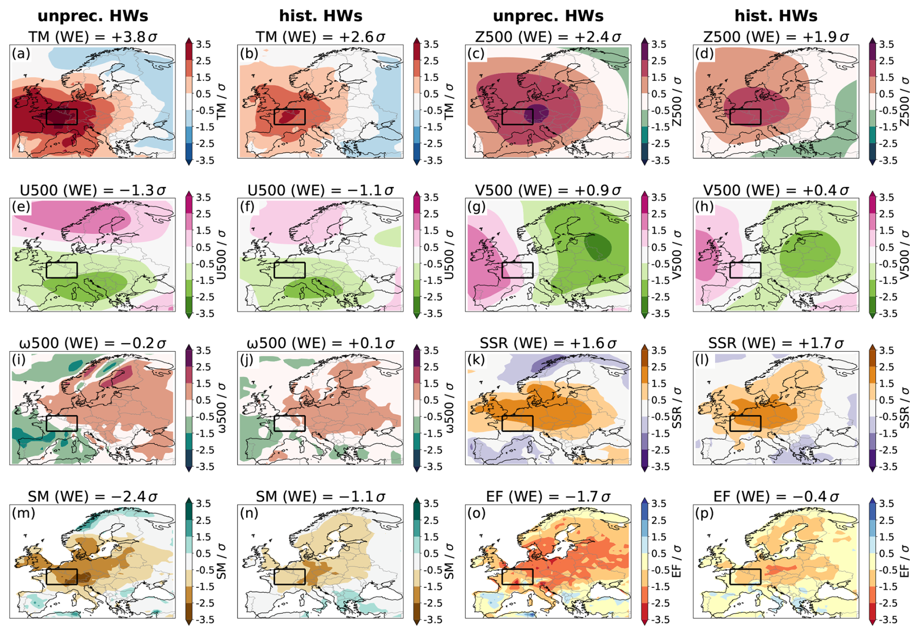
Figure 2 Spatial composites of anomalies in selected variables during unprecedented heatwaves (first and third columns) and during historical heatwaves (second and fourth columns). The surface variables SM and EF are only plotted over land.

First, the TM anomalies feature similar spatial distributions, extending slightly further west during unprecedented heatwaves (Fig. 2a and b). Similarly, the anomaly fields of the dynamical variables (Z500, U500, V500, and ω500) are also very similar between unprecedented and historical heatwaves, with very similarly located anticyclones over Central Europe that disturb the zonal flow over Central and Southern Europe, and lead to Southerly wind anomalies over Western Europe and above-average vertical subsidence over much of Central and Eastern Europe (Fig. 2c–j). The magnitudes of the anomalies are greater during unprecedented heatwaves, which is discussed in more detail in Sect. 3.2. The largest SSR anomalies are found in areas of vertical subsidence and are very similar in magnitude during historical and unprecedented heatwaves (Fig. 2k and l).

The fields of SM and EF feature substantially more negative anomalies in large parts of Central and Eastern Europe during unprecedented heatwaves (Fig. 2m–p; see also Sect. 3.2). Despite these differences in magnitude, the spatial distributions are still similar, with the most negative values of both SM and EF occurring to the east of WE, consistent with previous findings (Noyelle et al., 2025b). Overall, the large-scale conditions during unprecedented heatwaves in WE thus appear to be remarkably consistent, both externally with historical heatwaves and internally by conforming to well-understood physical processes. However, this good agreement in standardised anomalies does not necessarily extend to the case of the underlying absolute values, which can be subject to model biases in the mean and variability of heatwave variables.

Therefore, to complement our anomaly-based analysis, we also analyse the spatial fields of absolute values during unprecedented heatwaves. For this, we compare them with “recent” heatwaves that have occurred during 2011–2026 and are not included in our anomaly time series due to their incomplete centred 31-year climatology. These heatwaves are among the most extreme heatwaves in terms of absolute TM and occur in a very similar background climate as most of our unprecedented heatwaves (Fig. 3; see Sect. 2.3). As mentioned above, the unprecedented heatwaves are on average almost 5 K warmer than most recent heatwaves (Fig. 3a and b). However, the 2026 heatwave exceeded the previous 30 d TM record by approximately 2 K, and was almost as extreme in 30 d TX as some unprecedented heatwaves (see Appendix  B and Fig. B3).

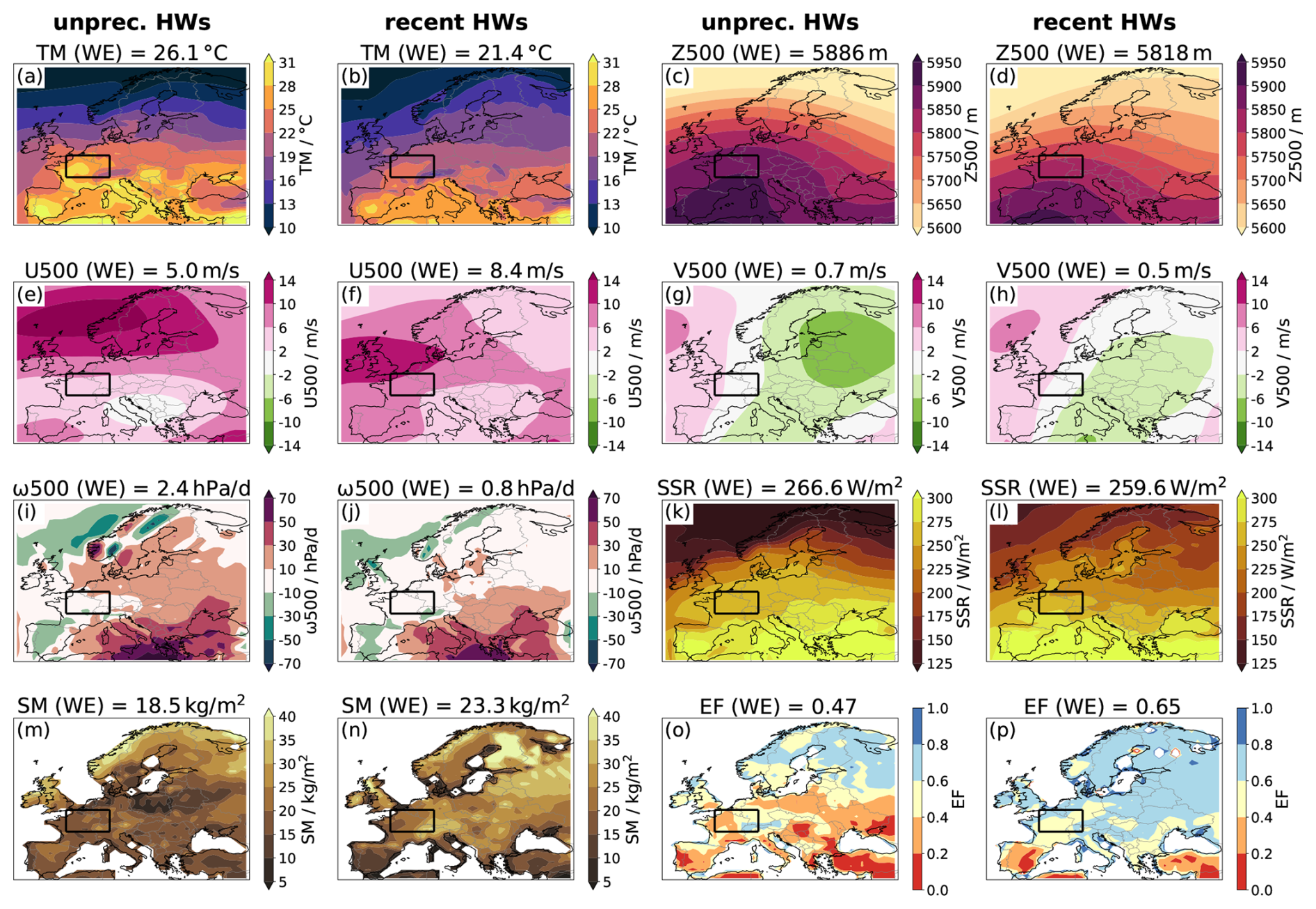
Figure 3 As Fig. 2, but for absolute values during unprecedented and recent heatwaves.

Apart from more extreme TM, unprecedented heatwaves are also associated with stronger anticyclones than recent heatwaves, but they are located in very similar positions (Fig. 3c and d). During unprecedented heatwaves, anticyclones extend further northward, which can also be seen in the location of the strongest zonal winds (Fig. 3e and f), while the positions of the strongest meridional winds are more similar (Fig. 3g and h). Both historical and unprecedented heatwaves feature the strongest vertical subsidence over South-East Europe and the Mediterranean, with much smaller values over WE (Fig. 3i and j). The northward shift of the strongest westerlies in the unprecedented heatwaves relative to the historical heatwaves can also be seen in the SSR, where the unprecedented heatwaves feature much lower values over Northern Europe (Fig. 3k and l). Some of the largest discrepancies are again visible in the surface variables SM and EF, whose absolute values are substantially lower across most of Europe during unprecedented heatwaves and which (in the case of SM) also exhibit different spatial patterns (Fig. 3m–p). However, it should be noted that these surface variables are associated with substantial uncertainties in both climate models and reanalysis, and thus absolute values in particular should be compared with caution (see Sect. 4).

In summary, absolute values during unprecedented heatwaves are much more extreme than recent heatwaves, not only in TM, but also in Z500, SM, and EF. Our analysis based on absolute values thus reveals similar differences between unprecedented and (recent) historical heatwaves as our anomaly-based framework. In addition, it also highlights differences in the meridional extent of the blocking anticyclone, which is greater in the unprecedented heatwaves. This indicates that CESM2 can simulate stronger blocking anticyclones than seen in the reanalysis record (see Sect. 3.4.3 for a more detailed discussion).

To conclude this section, the spatial fields of unprecedented heatwaves are very similar to those of historical heatwaves in anomaly space but, unsurprisingly, exhibit more discrepancies compared to recent heatwaves in their absolute values. This shows that unprecedented heatwaves appear to exhibit physically plausible large-scale conditions of heatwave driver anomalies, while the absolute values of these drivers should be interpreted with caution. In other words, plausibility in anomalies does not imply plausibility in absolute values, highlighting the importance of performing bias correction when using model output for impact assessment (Lüthi et al., 2024).

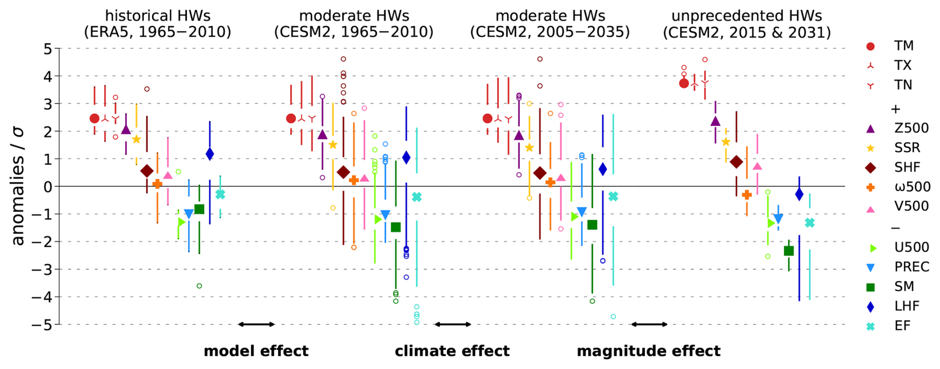
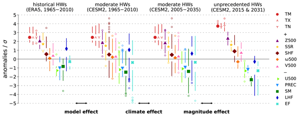
Figure 4 Anomalies of monthly mean heatwave variables in WE. Box plots of anomalies during historical heatwaves (HWs), moderate heatwaves from two different background climates, and unprecedented heatwaves: Median (filled symbols), inter-quartile range (IQR, empty space), whiskers (1.5 IQR, solid lines) and outliers (empty circles). We further indicate below the isolated effects of varying model, climate, and magnitude of heatwaves, respectively. For clarity of visualization, we broadly distinguish temperature variables (red), and variables with expected positive (“+”) and negative (“−”) anomalies during heatwaves.

3.2 Regional anomalies

As a next step, we analyse the monthly-mean anomalies in relevant heatwave variables during unprecedented heatwaves and compare them with the most extreme historical heatwaves (Appendix C, Fig. 4). For this, we focus on the 30 d anomalies of these variables averaged over WE. In this analysis, results that would indicate plausibility include (1) similar dominant drivers during historical and unprecedented heatwaves and (2) temperature anomalies whose magnitudes are consistent with the magnitudes of relevant drivers (for example, large temperature anomalies being associated with large anomalies in key drivers). In contrast, findings that would question the plausibility of these unprecedented heatwaves include (1) systematically different dominant drivers in historical and unprecedented heatwaves and (2) temperature anomalies whose magnitudes are decoupled from the magnitudes of relevant drivers (for example, large temperature anomalies being associated with only small anomalies in key drivers).

Overall, historical and unprecedented heatwaves are governed by quite similar dominant drivers, with large positive anomalies in Z500 and SSR and substantial negative anomalies in U500, PREC, and SM. In contrast, anomalies in SHF, ω500 (which we use as a proxy for adiabatic warming) and V500 (which we use as a proxy for mid-tropospheric temperature advection) appear to play a secondary role in both historical and unprecedented heatwaves. This relatively minor role for advective and adiabatic processes is partly caused by our focus on monthly-mean regional anomalies in this section, which can obscure short-term anomalies in these drivers (see Sect. 3.4.2). To disentangle and quantify the effects of these processes more explicitly, we also perform a temperature budget analysis (Sect. 3.4.1).

The main differences between historical and unprecedented heatwaves can be seen in variables related to land-atmosphere exchanges. In relative terms, SM and EF appear to play a substantially more important role during the unprecedented heatwaves than during the historical heatwaves. Furthermore, the anomalies in LHF are generally positive in historical heatwaves but mostly negative in unprecedented heatwaves. So what exactly explains these differences?

The unprecedented heatwaves structurally differ from the historical heatwaves in three main ways: They originate from a climate model rather than reanalysis, occur in a different background climate, and are more extreme in magnitude. To disentangle these effects on the anomalies of heatwave drivers, we additionally analyse “moderate” heatwaves simulated by CESM2 that have the same magnitude as historical heatwaves and are selected separately for two different climate periods (“historical” 1965–2010 and “present” 2005–2035; see Sect. 2.3). This allows us to distinguish between the three main effects at play:

(1) The “model effect”. Most physical drivers have similar anomalies during ERA5 and CESM2 heatwaves from the same climate. The CESM2 heatwaves have slightly less positive anomalies in Z500, SSR, SHF, and LHF and more negative anomalies in SM, but only the latter difference exceeds ±0.5 σ. This suggests that, when comparing heatwaves of the same magnitude from the same background climate, CESM2 generally captures the physical drivers present during heatwaves in ERA5 well. However, it also shows that CESM2 overestimates the role of drying soils during heatwaves. This finding is consistent with the literature (Vogel et al., 2018; Röthlisberger et al., 2026) and will be a theme throughout this work (see Sect. 3.4).

(2) The “climate effect”. Almost all physical drivers feature very similar anomalies during moderate CESM2 heatwaves from the historical and present climates, respectively. The only noticeable difference concerns LHF which exhibits anomalies of both signs in both background climates, but is shifted towards fewer positive and more negative anomalies in the present climate. Notably, this shift is not accompanied by a shift towards more negative SM anomalies, which might be expected from physical process understanding. However, the median of absolute SM values during moderate heatwaves is around 10 % lower in the present climate than in the historical climate (not shown). This is consistent with the projected long-term decrease in SM in Western Europe (Seneviratne et al., 2010), which is not visible in the anomalies due to our use of a time-evolving climatology. This means that the same SM anomaly can imply that land-atmosphere fluxes are energy-limited during historical heatwaves (causing more positive LHF anomalies), but transitional or even moisture-limited in present or future heatwaves (causing less positive LHF anomalies; Seneviratne et al., 2010). Between the historical and present climates compared here, this effect is still small, but it might become more substantial for future climates that see even stronger soil drying.

(3) The “magnitude effect”. The TM anomalies are >1 σ more extreme in the unprecedented heatwaves compared to the moderate heatwaves. As expected, this is accompanied by more extreme anomalies in most relevant drivers (Z500, SHF, V500, U500, PREC, SM, and EF); only SSR and ω500 exhibit unchanged and slightly less extreme anomalies, respectively. For LHF, the median anomalies in the unprecedented heatwaves are approximately 1 σ lower than during the moderate heatwaves, causing a switch from positive to negative median anomalies. This magnitude effect on LHF is noticeably greater than the combined model and climate effects, suggesting that the more negative SM anomalies are primarily responsible for the difference in LHF between historical and unprecedented heatwaves.

However, the shift from energy-limited to moisture-limited conditions also appears to have an effect among the unprecedented heatwaves themselves. The absolute values of SM are on average more than 15 % lower in the unprecedented heatwaves occurring in model year 2031 (parent ensemble P2) than in the other unprecedented heatwaves occurring in model year 2015 (parent ensemble P1, see Fig. B1c). This is presumably why their LHF anomalies are much more negative despite only slightly more negative SM anomalies (see, for example, U4 and U8 in Fig. B2b). This highlights an important limitation of our anomaly-based framework when comparing SM anomalies in different background climates, as this approach cannot capture non-linear behaviour such as changes in the regime of land-atmosphere interactions. At the same time, it also highlights the value of explicitly analysing anomalies in SHF, LHF, and EF, because these variables contain valuable information about the land-atmosphere interaction regime.

What conclusions does this analysis allow us to draw regarding the plausibility of unprecedented heatwaves? During historical, moderate, and unprecedented heatwaves, the largest anomalies consistently occur in the same physical drivers, most notably Z500, SSR, U500, and SM, and the unprecedented heatwaves feature more extreme anomalies in these drivers than the less extreme historical heatwaves (Fig. 4c). This implies that these unprecedented heatwaves are caused by “extreme anomalies of common drivers” (Fischer et al., 2021). This indicates that these heatwaves are internally consistent within CESM2 and also have external empirical support from historical precedent in ERA5. We also find that physically plausible, non-linear regime shifts in land-atmosphere interactions can limit the comparability of SM anomalies for future climate states.

3.3 Relationships between variables

The previous analysis has demonstrated that the relevant drivers of unprecedented heatwaves are similar to those during less extreme heatwaves in both CESM2 and ERA5. To further assess the internal consistency and physical conformity of these heatwaves, we now study the bivariate and multivariate relationships between relevant heatwaves variables. This allows us to test whether these variables follow well-known physical principles that govern their intervariate relationships and whether anomalies in different drivers are internally consistent.

3.3.1 Bivariate relationships

We first investigate the bivariate relationships between different relevant physical variables. For this, we select the annual JJA maxima in 30 d z_TM in ERA5 (1965–2010, 45 heatwaves) and CESM2-LE (2005–2035, 3100 heatwaves). We then compare the bivariate distributions of the 30 d anomalies in heatwave variables during unprecedented heatwaves with those during heatwaves in ERA5 and CESM2-LE (Figs. 5 and 6). Unprecedented heatwaves for which knowledge of the bivariate distributions in ERA5 and CESM2-LE and the anomaly in a given variable provides a good estimate of the anomaly in a second variable are considered plausible from a bivariate perspective. Conversely, obvious visual outliers from the mentioned bivariate distributions can count against plausibility of a given unprecedented heatwave if they cannot be explained by the behaviour of a third variable.

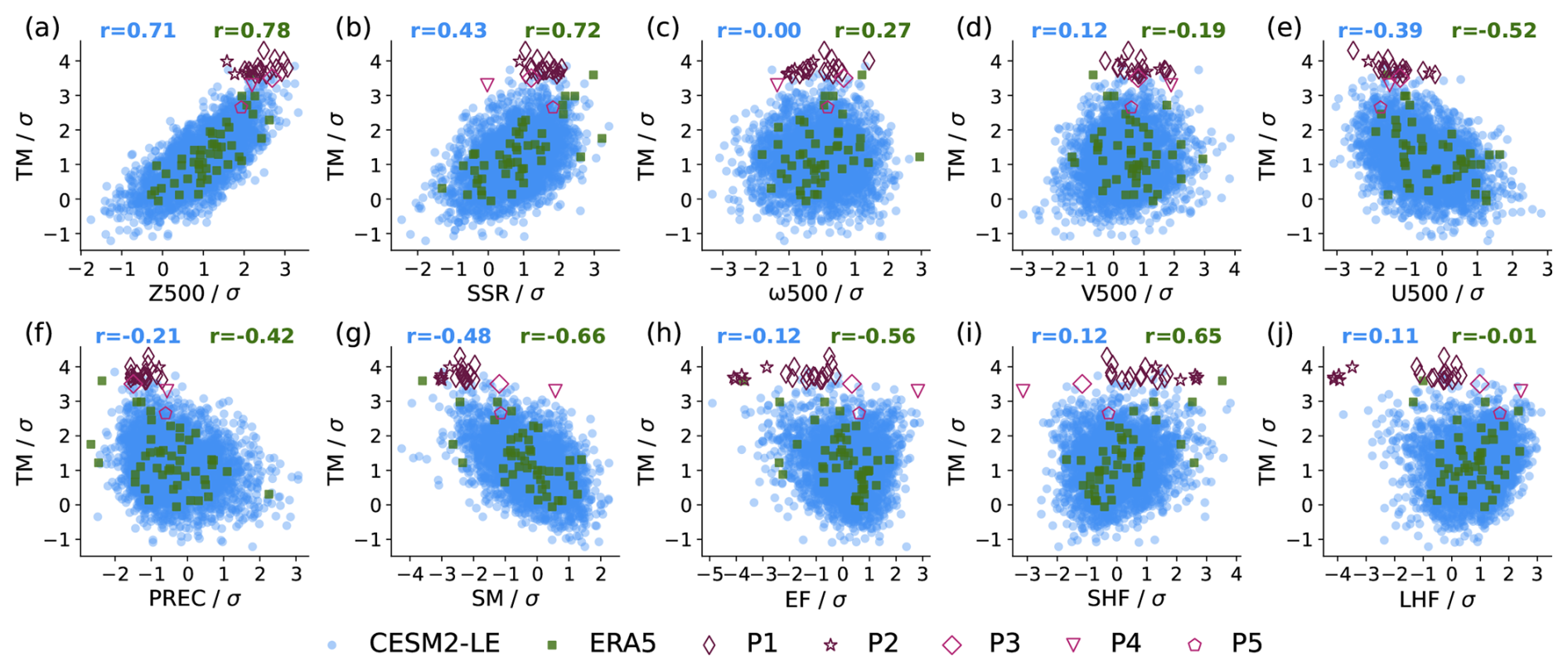
Figure 5 Bivariate distributions between TM and analysed heatwave drivers. Shown are the annual JJA maxima of 30 d temperature anomalies in CESM2-LE (2005–2035, blue circles) and ERA5 (1965–2010, green squares), as well as the 30 d anomalies during unprecedented heatwaves (purple) and precedented heatwaves (pink). The respective correlation coefficient r is noted at the top of the panel for CESM2-LE heatwaves (blue) and the ERA5 heatwaves (green).

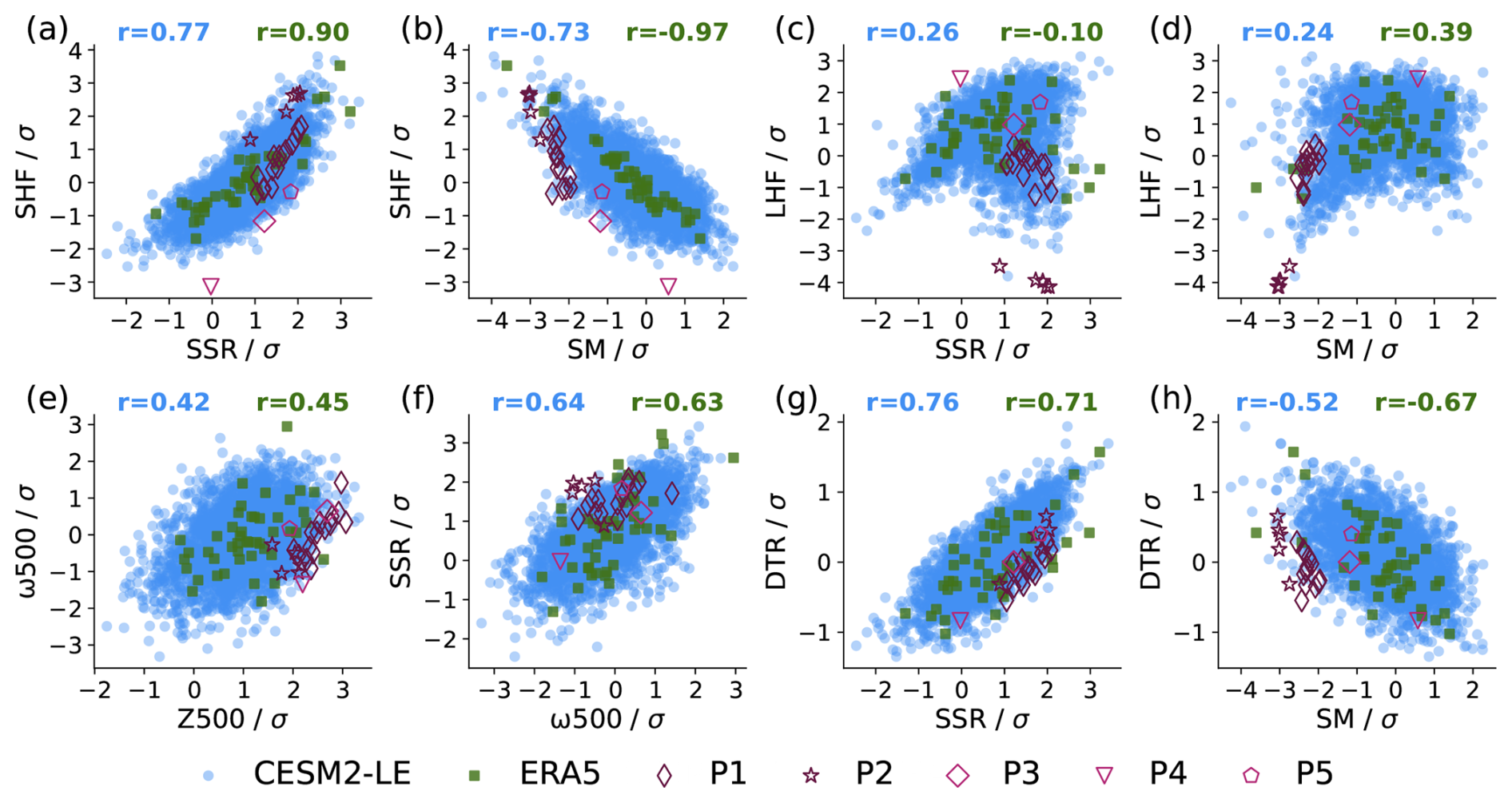
Figure 6 Same as Fig. 5, but for selected cross-relationships between different heatwave drivers and characteristics.

By definition, all unprecedented heatwaves have more extreme TM anomalies than heatwaves in ERA5 and almost all heatwaves in CESM2-LE, placing them at the upper edge of all bivariate distributions involving TM (Fig. 5). The different physical drivers can be broadly grouped into three different categories.

(1) Several drivers exhibit rather high correlations with TM, and their anomalies during precedented and unprecedented heatwaves are generally at the extreme ends of the CESM2-LE and ERA5 distributions. This is the case for Z500 (Fig. 5a), U500 (Fig. 5e), SM (Fig. 5h) and, to a lesser extent, PREC (Fig. 5f). These correlations align with physical process understanding, highlighting the importance of blocking anticyclones and drought conditions during heatwaves. Furthermore, the anomalies of these drivers are consistent with other heatwaves in CESM2-LE, but also with historical heatwaves in ERA5.

(2) Anomalies in ω500 (Fig. 5c) and V500 (Fig. 5d) have weak correlations with TM. For V500 this is not surprising given that temperature advection, by definition, mostly occurs non-locally. For ω500, this is contrary to the expectation that more extreme heatwaves would be associated with stronger sinking motion. This is presumably again because the 30 d mean can average out short periods of vertical subsidence or southerly wind (see Sect. 3.4.2). Furthermore, the regional anomalies on a single vertical level do not capture the full effect of these processes; for example, the signal can be more pronounced on other vertical levels (Hotz et al., 2024). Indeed, our temperature budget analysis at the 850 hPa level reveals substantial adiabatic sinking during unprecedented heatwaves (Sect. 3.4.1). Nevertheless, the near-zero ω500 anomalies of many precedented and unprecedented heatwaves are quite similar to the behaviour of heatwaves in CESM2-LE and ERA5 and consistent with anomalies in Z500 and SSR (Fig. 6e and f).

(3) The relationships of the surface heat flux variables with TM differ between CESM2 and ERA5. For EF and SHF, CESM2 shows a much weaker correlation with T2M than ERA5 (Fig. 5h and i). During almost all precedented and unprecedented heatwaves, SHF follows the strongly linear relationships with SSR and SM seen in ERA5 and CESM2-LE (Fig. 6a and b). The only exception is P4, presumably due to the combined occurrence of low SSR anomalies and high SM anomalies, both of which directly affect SHF, but whose individual contributions alone are not enough to explain the large negative SHF anomaly. In contrast, both CESM2 and ERA5 show very weak correlations between LHF and T2M, but tend to show heteroscedastic behaviour: Average TM anomalies feature a smaller spread in LHF than the most extreme TM anomalies, consistent with the fact that LHF anomalies vary strongly among the unprecedented heatwaves (Fig. 5j). This behaviour is not surprising given that surface fluxes strongly differ between moisture-limited and energy-limited conditions; during extreme conditions, this can be amplified through land-atmosphere feedbacks. LHF also features strong non-linearities in its relationships with SSR and SM in CESM2 and ERA5 (Fig. 6c and d). Most precedented and unprecedented heatwaves fall within the phase space covered by CESM2-LE and ERA5, but heatwaves from the parent ensemble P2 (model year 2031) fall outside the range covered by ERA5 and are only similar to a single heatwave in CESM2-LE, presumably due to their lower absolute values in SM (Sect. 3.2).

The only variable that does not nicely fall into any of the three mentioned categories is SSR, which shows a substantial positive correlation with TM, particularly in ERA5 (Fig. 5b). The SSR anomalies during the unprecedented and most precedented heatwaves align with the most extreme heatwaves in CESM2-LE; however, they are noticeably less extreme than expected from the bivariate distribution in ERA5. This could be caused by differences in cloud fraction or aerosol concentration (see Sects. 3.4.1 and 3.4.2). Nevertheless, the behaviours of other variables appear to be mostly consistent with relatively weak SSR anomalies, most notably the anomalies in SHF (Fig. 6a), ω500 (Fig. 6f) and DTR (Fig. 6g). Finally, the small SSR anomalies during unprecedented heatwaves are also presumably the reason why their DTR anomalies are smaller than expected from the SM anomaly alone (Fig. 6h).

In conclusion, most of the bivariate relationships analysed are consistent with the bivariate distributions seen in heatwaves in both CESM2-LE and ERA5, indicating that they are plausible from a bivariate perspective. In cases where this is not the case, the discrepancies propagate to other variables in a physically consistent way. This primarily concerns variables related to land-atmosphere interactions, which should be interpreted with caution given their substantial uncertainties in both CESM2 and ERA5/ERA5-Land. Furthermore, these discrepancies in part simply reflect changes in the land-atmosphere regime under climate change rather than physical inconsistencies. However, given the fact that many variables depend on more than one other variable, the bivariate approach is inherently limited in its ability to reliably detect multivariate outliers. This is therefore studied more thoroughly below.

3.3.2 Multivariate relationships

We now investigate how consistent the TM anomalies during the unprecedented (and precedented) heatwaves are given the combinations of anomalies in multiple different drivers. To this end, we employ a simple multilinear statistical model that infers the 30 d temperature anomaly based on the 30 d anomalies in five physical drivers: Z500, U500, V500, SM, and SSR. This selection is to some extent inherently arbitrary; it represents a compromise between model simplicity, predictor independence, and explained variance (see Sect. 2.6). We use six different versions of the multilinear model, separately trained to infer TM, TX, and TN based on heatwaves in CESM2-LE and ERA5, respectively. These different model versions are used to infer 30 d anomalies in TM, TX, and TN during precedented and unprecedented heatwaves based on anomalies in the five predictors (Fig. 7). The CESM2-LE trained model is primarily used to assess internal consistency, while the ERA5 trained model evaluates whether the processes during these heatwaves are in line with those during historical heatwaves in reanalysis.

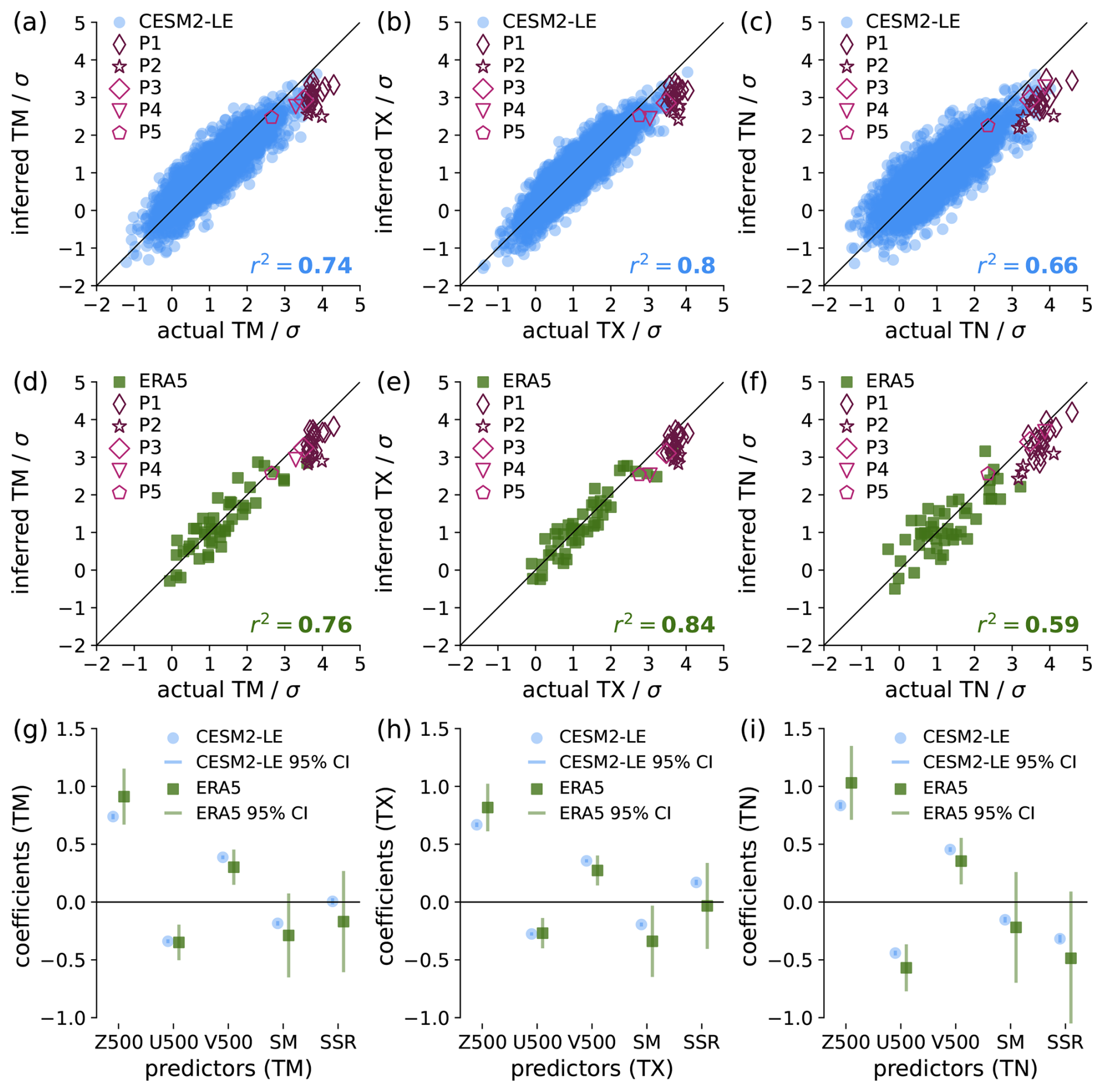
Figure 7 Actual anomalies of TM (a, d), TX (b, e), and TN (c, f) and anomalies inferred using our multilinear statistical model. Shown are the training data, namely the annual maxima of 30 d TM anomalies in WE during the summer season (JJA) in CESM2-LE (a–c, blue circles) and in ERA5 (d–f, green squares), respectively. The model is applied to 30 d anomalies of TM, TX, and TN in WE during unprecedented heatwaves (purple) and precedented heatwaves (pink). For reference, the 1:1 line and the explained variance r² of each model are also shown. The regression coefficients of each predictor and their 95 % confidence intervals (CI) are compared for TM (g), TX (h), and TN (i).

If both the CESM2-LE and ERA5 trained models are able to infer the temperature anomalies of unprecedented heatwaves based only on anomalies of the five drivers, this suggests that the magnitudes of these heatwaves are explained by well-established physical processes that behave linearly even outside the training data and across different models, supporting plausibility. Conversely, non-linearities of land-atmosphere interactions discussed above could cause some discrepancies between actual and inferred temperature anomalies. However, the model should still be able to infer a large fraction of the temperature anomaly from the other drivers (and the linear component of SM), particularly given the high explained variance within the training data. Therefore, substantial overestimations or underestimations of temperature anomalies by a model would question the plausibility of the heatwave from a multivariate perspective. In this way, the multilinear model serves as a more quantitative and holistic assessment of plausibility from a multivariate perspective compared to the more qualitative, bivariate assessment in the previous section.

Our multilinear models capture 80 %–85 % of the variance in TX, 75 % in TM, but only 60 %–65 % of the variance in TN. The lowest explained variance in TN is not surprising, because it is more strongly affected by processes not directly captured in our model, such as the downwelling longwave radiation from water vapour and clouds. Although our models explain the majority of the variance in the training data and thus perform well on average, they tend to underestimate the magnitude of the most extreme heatwaves, both for the training data and the (un)precedented heatwaves to which they are applied. This is not surprising given that (1) the models are trained to perform well in the most extreme heatwave in an average summer and are thus affected by regression to the mean, and (2) our simple least-squares approach neglects uncertainty in the independent variable and is thus sensitive to regression dilution (Pitkänen et al., 2016). This behaviour is further favoured by the strongly non-linear nature of land-atmosphere interactions and our omission of several relevant variables to achieve model simplicity. However, the main goal here is not to perfectly capture all processes affecting TM anomalies, but rather to assess whether the unprecedented heatwaves behave similarly in a multivariate phase space compared to other heatwaves in climate models and reanalysis. In Fig. 7, this corresponds to the question whether the data points of the unprecedented heatwaves behave consistently with the most extreme heatwaves in the training data.

In general, precedented and unprecedented heatwaves behave remarkably similarly to heatwaves in both CESM2-LE and ERA5. Although their magnitudes are underestimated by our models, this underestimate is similar to the underestimate of the most extreme heatwaves in the training data. For some heatwaves from parent P2, the magnitudes are underestimated more strongly than comparable heatwaves in the training data; however, the magnitude of the deviation from the 1:1 line is still comparable to the differences found for less extreme heatwaves in the training data. This underestimate is presumably related to non-linear shifts in the land-atmosphere interaction regime, as discussed in Sect. 3.2. Five of the six models include training data heatwaves of comparable magnitude to the unprecedented heatwaves, that is, the anomalies during the unprecedented heatwaves only slightly exceed the most extreme heatwave in the training data. However, the TN anomalies of many unprecedented heatwaves are far more extreme than any heatwave in ERA5 (Fig. 7f). Despite this fact, the ERA5 trained model only slightly underestimates the TN anomalies of the unprecedented heatwaves. This shows that these unprecedented heatwaves are governed by processes very similar to those of historical heatwaves.

Another way to assess plausibility from a multivariate perspective is through the model coefficients (Fig. 7g–i). In general, the differences in coefficients between the different prognostic variables exhibit physically reasonable behaviour. For example, the SSR coefficient is most positive for TX and most negative for TN, presumably due to the associated lower nighttime cloud cover. These two effects appear to largely cancel, which is why the effect of SSR on TM is much smaller than that of the other variables analysed. Furthermore, SM seems to play a larger role for TX than for TN, presumably as a result of surface heat fluxes induced by solar heating during the day. In contrast, the coefficients of the adiabatic and advective variables (Z500, U500, V500) are much stronger for TN than for TX. The coefficients for the models trained on CESM2-LE and ERA5 are generally similar and lie within their respective 95 % confidence intervals. Compared to ERA5, CESM2 has less positive Z500 coefficients, more positive V500 coefficients, less negative SM coefficients, and systematically higher SSR coefficients (more positive for TX, less negative for TM and TN). However, these differences should not be overinterpreted, given the large confidence intervals for the ERA5-trained model, caused by the small sample size and the high collinearity between SSR and SM in ERA5 (not shown).

To further investigate the role of non-linearities in land-atmosphere fluxes, we use the same model setup to predict SHF, LHF, and EF based on TM, SM, and SSR (see Sect. 2.6, Fig. B4). For SHF, the multilinear models capture 80 %–90 % of the variance in the training data, a surprisingly high value given that the models do not contain information on the near-surface wind (Fig. B4a and d). The CESM2-LE trained model performs decently in inferring SHF during (un)precedented heatwaves, while the ERA5 trained model systematically overestimates SHF during these heatwaves. For LHF, the multilinear model only explains 40 %–60 % of the variance (Fig. B4b and e). This is presumably due to missing information about near-surface wind and humidity and due to non-linearities between SM and LHF, visible from the strong deviations from the 1:1 line at large negative LHF anomalies for the CESM2-LE model in particular. These effects also affect EF, but to a somewhat lesser extent (Fig. B4c and f).

These multivariate models confirm that the surface fluxes during the precedented heatwave P4, which lie outside the respective bivariate distributions, are predicted reasonably well by the CESM2-LE trained model, but not by the ERA5 trained model – not surprising given different parametrisations of surface fluxes in CESM2 and ERA5. This is also apparent from the very different model coefficients of our multilinear model (Fig. B4g–i), demonstrating that, even in anomaly space, one should be careful in directly comparing them. Given the comparatively poor performance of our multilinear models in inferring surface fluxes during precedented and unprecedented heatwaves, it is remarkable that our models perform as well as they do in inferring temperature anomalies during the same heatwaves. This is particularly notable for the ERA5 trained model, given the demonstrated discrepancies in the treatment of surface fluxes compared to CESM2. This demonstrates that, despite the presence of non-linearities in land-atmosphere interactions, temperatures during unprecedented heatwaves can be well explained by a linear combination of five predictors. This solidifies that it is in fact “extreme anomalies of common drivers” acting in an approximately linear way to cause these heatwaves.

In summary, all of our model versions can infer temperature anomalies during the unprecedented heatwaves with accuracies similar to those in the training data. This suggests that the linear combination of five drivers can explain most of the magnitude of the unprecedented heatwaves, and that, even very far in the tail, non-linearities appear to play a secondary role. Within CESM2, this is not entirely surprising, but, given substantial tuning to represent the mean climate state, it is still an important finding that internal consistency of physical processes still holds for extremes far in the tail. Remarkably, this consistency even applies to model versions trained only on historical heatwaves in ERA5, showing that the multilinear model is robust across training data from different physical models. We can thus conclude that, although these unprecedented heatwaves are far more extreme than the most extreme historical heatwaves, they appear to be internally consistent and have external empirical support from a multivariate perspective.

3.4 Temporal substructure

The analyses above have exclusively focused on temporal averages over the entire 30 d durations of the unprecedented heatwaves. While this contains valuable information about the mean state during these heatwaves, it can average out variations on shorter time scales, and is thus inherently limited in fully assessing the relevant underlying processes. In the following, we therefore focus on the temporal substructure of unprecedented heatwaves on the daily timescale.

3.4.1 Temperature budget analysis

First, we perform a Eulerian temperature budget analysis at the 850 hPa level, disentangling the advective, diabatic, and adiabatic contributions to historical and recent heatwaves in ERA5 and to precedented and unprecedented heatwaves in CESM2 (Fig. 8, see Sect. 2.4). In this analysis, the plausibility of unprecedented heatwaves would be confirmed by local temperature tendencies that occur due to similar physical processes, whereas it would be questioned for substantially different underlying processes. We average the tendencies separately for days with increasing local temperature (“warming days”, Fig. 8a) and decreasing local temperature (“cooling days”, Fig. 8b). Because the analysis is based on absolute values rather than anomalies, it is subject to systematic model biases. However, the local tendencies during the heatwaves analysed are generally quite similar, allowing for a comparison of the relative importance of the underlying processes.

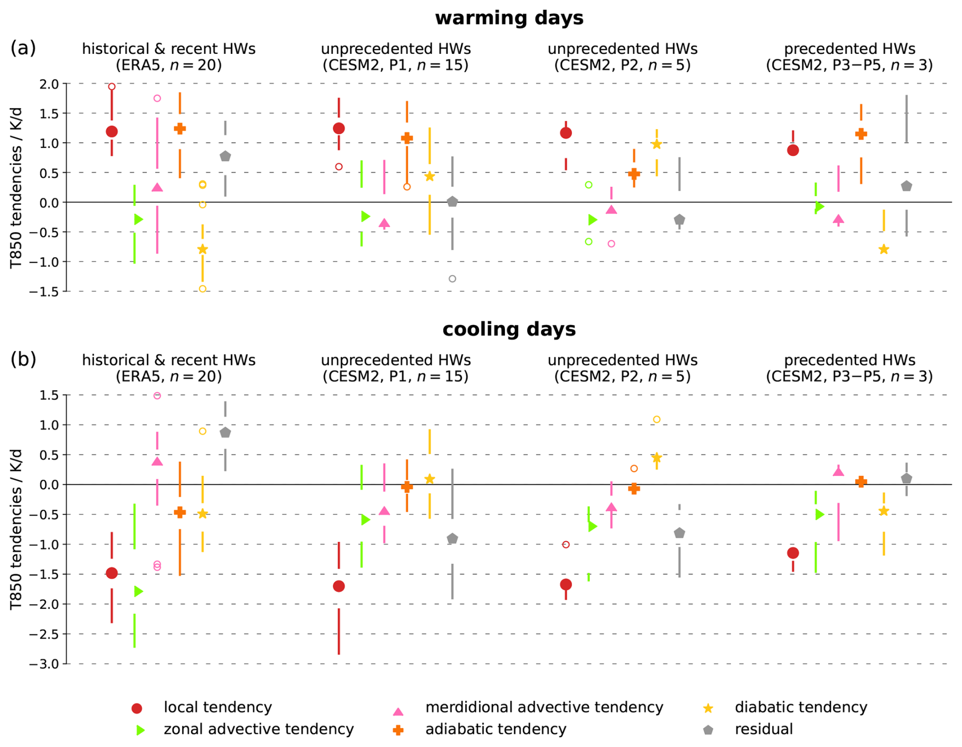
Figure 8 Tendencies of 850 hPa temperature (T850) during historical and recent heatwaves in ERA5, as well as precedented and unprecedented heatwaves in CESM2, shown separately for different parent ensembles. Shown are the terms of Eq. (2), averaged over each event during days with positive (a) and negative local T850 tendency (b): Median (filled symbols), inter-quartile range (IQR, empty space), whiskers (1.5 IQR, solid lines) and outliers (empty circles).

During warming days, unprecedented heatwaves feature weaker adiabatic warming than ERA5 heatwaves. This difference is small for heatwaves from the P1 ensemble, but exceeds 50 % for the five heatwaves from the P2 ensemble. During the three precedented heatwaves P3–P5, the adiabatic contribution is very similar to the ERA5 heatwaves. Conversely, there is net diabatic cooling during ERA5 heatwaves, presumably dominated by longwave radiation and evaporation, but net diabatic warming during unprecedented heatwaves. This is particularly pronounced for P2 heatwaves, consistent with their extreme anomalies in SM and SHF, while the precedented heatwaves P3–P5 feature net diabatic cooling, consistent with their much less extreme anomalies in SM and SHF (Fig. 5i). The zonal and meridional advective tendencies are smaller in magnitude, with ERA5 heatwaves featuring net meridional warming rather than cooling, but also non-negligible positive residuals.

During cooling days, temperature tendencies are dominated by advective cooling, but while ERA5 heatwaves feature strong zonal cooling and weak meridional warming, unprecedented heatwaves feature weak zonal and meridional cooling. Again, precedented heatwaves are more similar to ERA5 heatwaves in this respect. Furthermore, CESM2 heatwaves feature close to zero adiabatic contributions, in contrast to substantial adiabatic cooling during ERA5 heatwaves. The diabatic tendencies are of smaller magnitude than during warming days, but feature the same discrepancies regarding their signs. However, the residual terms are substantial and of opposite sign, and thus these results should be interpreted with caution.

Overall, we find that the unprecedented heatwaves in CESM2 are caused by stronger diabatic and weaker adiabatic tendencies than historical heatwaves in ERA5. This is in line with the findings of Röthlisberger et al. (2026) who found biases of CESM2 relative to ERA5 based on Lagrangian backward trajectories that are consistent with the differences found here. However, the less extreme precedented heatwaves feature much more similar contributions compared with ERA5, indicating that these results depend on the exact heatwaves analysed. Nevertheless, these discrepancies in the processes that cause unprecedented heatwaves in CESM2 casts some doubt on their physical conformity. Because the discrepancies mainly concern the relative contributions of diabatic vs. adiabatic terms, some of this can compensate to still yield similar behaviour in temperature, as discussed below.

3.4.2 Rank anomalies

Next, we rank the daily anomalies of heatwave variables from highest to lowest within the 30 d historical, moderate, and unprecedented heatwaves (Fig. 9), similar to the approach of Röthlisberger et al. (2020). Because we rank the anomalies separately for each variable, the ranked days of the different variables do not correspond to each other. To be plausible, unprecedented heatwaves should feature similar relationships between the most extreme and least extreme daily anomalies as historical and moderate heatwaves. In contrast, unprecedented heatwaves dominated by only a few days of outliers would be considered less plausible. For this analysis, we only consider the model effect (ERA5 vs. CESM2) and the magnitude effect (moderate vs. unprecedented heatwaves) but not the much smaller climate effect (historical vs. present climate; see Sect. 3.2). Thus, we only include moderate heatwaves from the present climate (2005–2035). The two effects are discussed below.

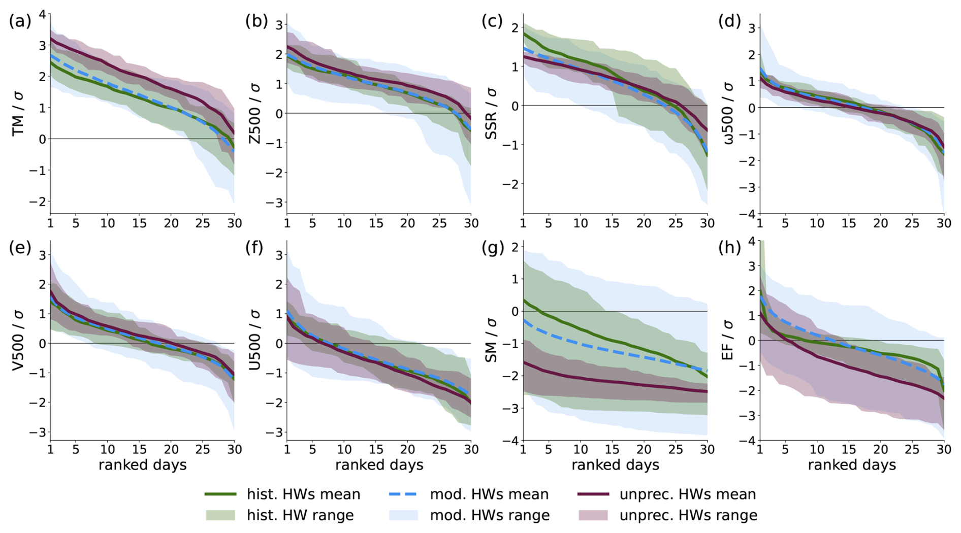
Figure 9 Ranked daily anomalies of heatwave variables. Shown are the mean (lines) and range (shading) during historical heatwaves (green), moderate heatwaves (blue), and unprecedented heatwaves (purple). Variables are sorted from highest to lowest anomalies, meaning that the most favourable conditions for heatwaves are found at low-ranked days in panels (a)–(e), but at high-ranked days in panels (f)–(h).

(1) The model effect: The temporal substructures of most variables are very similar during historical and moderate heatwaves of the same magnitude (TM, Z500, ω500, V500, and U500; Fig. 9a, b, d, e, and f), with three notable exceptions. (a) SSR anomalies on the sunniest days are less positive in moderate heatwaves (ranked days 1–15 in Fig. 9c). As discussed above, this is presumably related to differences in cloud fraction, indicating that even on the sunniest days, CESM2 might still simulate some cloud cover. It might also be affected by different aerosol concentrations, as aerosol-radiation interactions are most important on days with low cloud cover. (b) SM anomalies on less dry days are more negative in the moderate heatwaves, suggesting discrepancies in the persistence of agricultural droughts in CESM2 (ranked days 1–20 in Fig. 9g; see Sect. 3.4.3). (c) EF anomalies exhibit more strongly positive and more strongly negative daily anomalies in moderate heatwaves, while most daily anomalies during historical heatwaves are much closer to zero (Fig. 9h). This discrepancy presumably reflects differences in the parametrisation of surface heat fluxes between ERA5 and CESM2.

(2) The magnitude effect: Features (a)–(c) appear to be model specific, as they can also be detected for the unprecedented heatwaves. In addition, unprecedented heatwaves unsurprisingly feature substantially greater daily TM anomalies throughout the 30 d period than moderate heatwaves, with a weaker shift on the coolest days (ranked days 25–30 in Fig. 9a). Most other variables also exhibit very similar daily anomaly distributions between moderate and unprecedented heatwaves (Z500, SSR, ω500, V500, and U500; Fig. 9b–f). For Z500, unprecedented heatwaves exhibit a shift of the ranked anomalies towards more positive values for days of weaker Z500, indicating more persistent anticyclones (ranked days 20–30 in Fig. 9b). For V500 and ω500, the temporal substructures reveal that their small 30 d mean anomalies are partially due to the long averaging period; short-term periods of southerly wind or vertical subsidence are largely cancelled out by periods of negative anomalies as the anticyclone itself moves (Fig. 9d and e). SM anomalies are more negative during unprecedented heatwaves throughout the 30 d periods, but particularly for less dry days (ranked days 1–20 in Fig. 9g). This suggests that it is the persistence of low SM, rather than the driest SM days, that makes the unprecedented heatwaves so exceptional. Interestingly, this behaviour is not mirrored by EF, whose shift towards more negative anomalies is strongest for days with intermediate and low EF anomalies (ranked days 10–25 in Fig. 9h), which might be partially explained by the smaller SSR anomalies on sunny days.

To assess how representative these results are, we repeat this analysis for the three precedented heatwaves from three different parent ensembles (Fig. B5). Although the small sample size means that the results should not be overinterpreted, we find that most variables again feature similar daily anomaly distributions (TM, Z500, ω500, V500, U500) and that the daily anomalies in SM and EF show the opposite behaviour of the unprecedented heatwaves, with uniform shifts to substantially less negative (or even positive) anomalies throughout their duration. This suggests that the much less dry soil is primarily responsible for the less extreme TM anomalies compared to the unprecedented heatwaves.

Overall, the temporal substructures of most variables are internally consistent within CESM2 and have external empirical support from historical precedent in ERA5. The most notable exception is the apparent overestimation of persistence in SM anomalies by CESM2, which will be analysed in more detail next.

3.4.3 Persistence

Finally, we evaluate the temporal persistence of relevant heatwaves variables, comparing the occurrence of periods in which the anomalies of TM and Z500 exceed +1 σ, and in which the anomalies of SM remain below −1 σ, respectively. For this, we compare precedented and unprecedented heatwaves with historical heatwaves, as well as with the JJA distributions of ERA5 and CESM2-LE (see Sect. 2.5). With this analysis, we assess the systematic differences between ERA5 and CESM2 and the position of the unprecedented heatwaves relative to the CESM2 distribution and the historical heatwaves. Findings that would support their plausibility include: (1) ERA5 and CESM2-LE exhibiting similar distributions, (2) the unprecedented heatwaves consistently remaining within CESM2-LE distribution, and (3) the persistence of the unprecedented heatwaves being higher than that of historical heatwaves, but still of roughly comparable magnitude. If one or more of these conditions are not met, this would argue against the plausibility of these heatwaves. For the persistence of TM, a systematic overestimation by CESM2 would count against plausibility, as it would indicate that a simulated heatwave occurs only due to model biases. In contrast, a systematic underestimation of TM persistence by CESM2 would not necessarily suggest the same, but might instead indicate that the persistence of real-world heatwaves could even exceed that of unprecedented heatwaves.

For Z500, CESM2 captures the frequencies of short persistence durations (<10 d) quite well, but it substantially underestimates the frequency of longer persistence durations (Fig. 10a). The discrepancy is even more pronounced when we compare the persistence of atmospheric blocking (Fig. 10b, Sect. 2.5). CESM2 strongly underestimates the occurrence of consecutive blocked days for short persistence durations and even more strongly for long persistence durations. This systematic underestimate of persistent atmospheric blocking regimes in CESM2 also seems to affect the unprecedented and precedented heatwaves. Although they tend to exhibit longer persistence durations with respect to 1 σ-threshold exceedances of Z500 anomalies than historical heatwaves, the picture is almost exactly reversed for consecutive blocked days, except for only the precedented P3 heatwave. This is consistent with previous findings that global circulation models (GCMs) struggle to reproduce persistent blocking regimes (Tibaldi and Molteni, 1990; Davini and D’Andrea, 2016; Liu et al., 2022).

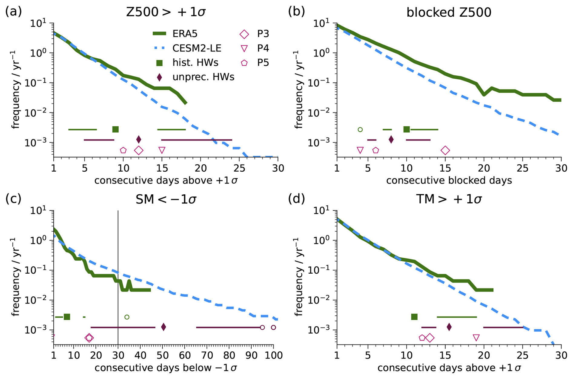
Figure 10 Persistence of selected heatwave variables. (a, c, d) Number of consecutive days in JJA with daily anomalies $\ge +\mathrm{1}\mathit{\sigma }$ (TM and Z500) or $\le -\mathrm{1}\mathit{\sigma }$ (SM). Shown are the relative frequencies in ERA5 (green) and CESM2-LE (blue), and box plots of values during historical heatwaves (green) and unprecedented heatwaves (purple): Median (filled symbols), inter-quartile range (IQR, empty space), whiskers (1.5 IQR, solid lines) and outliers (empty circles). The values during the precedented heatwaves from other parent heatwaves are also shown (pink symbols). Note the different x axis for SM in panel (c). (b) As panel (a), but showing the number of consecutive blocked days (Sect. 2.5.)

The opposite phenomenon can be seen for SM, where CESM2 simulates a higher frequency of long persistence durations (>15 d). Furthermore, while precedented heatwaves feature persistence durations comparable to historical heatwaves, unprecedented heatwaves feature persistence durations up to three times longer (Fig. 10c). Presumably, this is at least partially because CESM2 simulates many more negative SM anomalies relative to ERA5-Land (Fig. B6). It is also consistent with the findings of Vogel et al. (2018) that climate models tend to overestimate soil drying due to land-atmosphere feedbacks. Furthermore, although monthly soil moisture memory is generally well represented in GCMs, there are substantial regional and intermodel differences (Seneviratne et al., 2006).

The net effect of these two processes can be seen in the persistence of TM, where CESM2 and ERA5 simulate very similar occurrences of short persistence durations (Fig. 10d). CESM2 underestimates the occurrence of longer persistence durations in TM, but the differences relative to ERA5 are smaller than for Z500 and SM. Despite this systematic underestimate, precedented and unprecedented heatwaves on average feature longer persistence durations in TM than historical heatwaves.

Overall, CESM2 struggles to accurately capture persistence durations relative to ERA5, with substantial discrepancies between the roles of diabatic contributions (related to persistence of SM) and adiabatic contributions (related to persistence of Z500), as already shown above. Thus, unprecedented heatwaves simulated by CESM2 occur for “partly the wrong reasons”, in line with previous findings (Röthlisberger et al., 2026). These limitations of CESM2 in simulating the physical processes causing long persistence durations consistently with historical precedent raise concerns regarding the physical conformity – and thus the overall plausibility – of the unprecedented heatwaves. Nevertheless, despite these discrepancies in the underlying processes, the discrepancies in the persistence of TM itself are comparatively smaller. Given that CESM2 underestimates the persistence of TM and only a few unprecedented heatwaves feature longer TM persistence durations than seen in the short reanalysis record, this suggests that heatwaves with comparable or even longer persistence of TM are plausible to occur in the real world, although with different roles for diabatic and adiabatic processes. In fact, we argue that these heatwaves might even represent a conservative estimate for worst-case long-lasting heatwaves in terms of their persistence in TM.

4 Discussion

Our assessment of plausibility is mostly based on standardised anomalies, which is essential to meaningfully compare extremes occurring in different background climates. By construction, this approach removes systematic differences in mean state and variability between CESM2 and ERA5. Thus, our assessment that extreme heatwaves simulated in CESM2 are plausible to occur in the real world refers primarily to standardised anomalies rather than to the absolute physical state. This means that even for plausible heatwaves, absolute values should be treated with caution, an important caveat given that impact studies are generally based on absolute thresholds rather than anomalies. Thus, it remains essential to perform a bias correction of the raw model output when model-based storylines are used for stress testing and disaster preparedness (Lüthi et al., 2024).

Although standardised anomalies correct for many model biases in mean state and variability, some systematic differences remain. Compared to observations, GCMs tend to overestimate soil drying during heatwaves due to differences in the representation of land-atmosphere feedbacks (Vogel et al., 2018). Furthermore, the atmospheric circulation in GCMs is too zonal, that is, GCMs systematically underestimate the occurrence and persistence of atmospheric blocking, a major driver of heatwaves (Tibaldi and Molteni, 1990; Davini and D’Andrea, 2016; Liu et al., 2022). These biases can partially compensate, leading to simulated heatwaves that occur for “partly the wrong reasons” (Sect. 3.4.1 and 3.4.3; Röthlisberger et al., 2026).

Furthermore, although we often refer to the non-temperature variables analysed as heatwave “drivers”, it is not always possible to cleanly separate cause and effect. For example, soil moisture can cause temperature anomalies, but can also be amplified by them through land-atmosphere feedbacks (Seneviratne et al., 2010). Therefore, one must be careful in asserting causality, especially at a monthly time scale. For this reason, we further analyse the partitioning of latent and sensible heat flux in the evaporative fraction and focus on internal consistency rather than causal relationships.

Another caveat concerns the use of monthly regional anomalies in V500, ω500, and SHF as proxies for temperature advection, adiabatic subsidence, and diabatic warming in some of our assessments. This neglects upstream and non-local processes, and vertical variations in the atmosphere (Hotz et al., 2024). For further studies, our approach could therefore be complemented by a more comprehensive analysis of the underlying atmospheric dynamics, for example, using Lagrangian backward trajectories or circulation-regime diagnostics (Röthlisberger and Papritz, 2023; Hochman et al., 2021). Our Eulerian approach is motivated by two main arguments: (1) It is much easier and less computationally expensive to implement and could therefore realistically be included in an operational assessment of plausibility (Kelder et al., 2022a). (2) The stationarity of the weather systems required to produce heatwaves on a monthly time scale makes the Eulerian approach much more suitable than for heatwaves or other extreme events occurring on shorter time scales.

In order to still gain more insights into the underlying processes, we perform a Eulerian temperature budget analysis, but this also comes with a few caveats: Our focus on the 850 hPa level reduces the effects of topography, but does not remove them. This leads to large residuals over mountain ranges, which is why we exclusively evaluate the temperature budget for the regional WE mean. Furthermore, focusing on the 850 hPa level presumably underestimates the diabatic contributions of land-atmosphere exchanges, which are strongest close to the surface. Furthermore, the systematically opposite signs of both the diabatic contribution and the residuals between CESM2 and ERA5 might reflect differences in the parametrisations underlying the diabatic tendencies. Finally, part of the non-negligible residual terms are presumably explained by our use of daily time steps, whereas the spatial resolution of the model output seems to play only a secondary role for the regional WE mean budget.

Evaluating historical precedent for heatwaves in a rapidly warming climate is inherently challenging, but is made possible by our approach of considering standardised anomalies relative to a time-evolving climatology. While useful, this view can in principle obscure the fact that the same anomaly might be plausible in past climates, but not necessarily in future climates. This is particularly true for non-negative variables that can exhibit substantial non-Gaussianity, such as PREC or SM, particularly when combined with a decreasing trend over time. But it can also complicate the interpretation of negative anomalies in U500, as it is not obvious whether they imply weaker-than-average westerlies or easterly winds. The time-evolving climatology itself is also subject to uncertainties; for example, a 30-year climatology is difficult to precisely constrain in regions with unusually warm or cold periods caused by internal variability. Nevertheless, it offers clear improvements in assessing the extremeness of an event relative to the climate in which it occurred compared to a climatology based on a fixed time period.

Another limitation concerns the inherently limited sample size of historical heatwaves in the reanalysis record. Some of this might be overcome by choosing a longer data set for reanalysis, such as the Twentieth Century Reanalysis (Compo et al., 2011). However, by their very nature, unprecedented heatwaves do not have precedents of comparable magnitude in reanalysis data sets, regardless of the covered time period. Furthermore, due to much sparser observations in the first half of the twentieth century, such reanalyses are much less constrained by observations and instead rely much more heavily on the underlying physical model, leading to additional uncertainties and potential biases.

For related reasons, it is important to be careful when comparing surface energy variables between CESM2 and ERA5. Although temperature and circulation variables in reanalysis are strongly constrained by observations, this constraint is much weaker for variables related to the surface energy budget, such as SHF, LHF, and SM. Instead, their values are strongly affected by the atmospheric and land surface models and parametrisations of land-atmosphere interactions used; furthermore, ERA5 fails to close the surface energy budget (Hersbach et al., 2020; Muñoz-Sabater et al., 2021). Therefore, reanalysis values of these variables should not be considered as “ground truth” but instead be interpreted cautiously. Our anomaly-based approach is designed to correct for many of these discrepancies, including biases in the mean and variance of surface variables, but not for differences in higher-order moments of the distributions.

We demonstrate the feasibility of our process-based plausibility assessment approach for heatwaves, because these are the extreme events with the most solid understanding of the underlying physical processes. In principle, our approach can also be applied to other extreme events, but it should be noted that the physical drivers of these events are less well understood and in some cases less straight-forward to implement in our framework. For example, it should be quite straight-forward to apply our approach to large-scale events that can be realistically simulated in general circulation models, such as cold spells or droughts. For smaller-scale events, such as heavy convective precipitation or wind storms, high-resolution modelling is required.

Finally, all unprecedented heatwaves analysed in this study are based on a single model. Given well-documented intermodel differences among GCMs, this inherently limits the generalisability of our results. Our approach presented here can serve as a blueprint for performing similar analyses with other models, which would be very valuable to allow conclusions to be made less dependent on the specific climate model. In particular, models that have already been used to create climate storylines should be evaluated in this way, which could provide a better picture of how plausible extreme heatwaves they simulate are.

5 Conclusions

We present a process-based approach to assess the plausibility of unprecedented climate storylines and apply it to month-long heatwaves in Western Europe that would exceed the most extreme historical heatwaves by more than 5 K. We compare 20 unprecedented month-long heatwaves in Western Europe from CESM2 ensemble boosting simulations with the most extreme historical heatwaves in ERA5 using standardised anomalies relative to a time-evolving climatology.

The unprecedented heatwaves are associated with physical drivers well-known from less extreme heatwaves in climate models and reanalysis, including strong anticyclones, low levels of soil moisture, and high values of surface solar radiation, demonstrating the physical conformity of these heatwaves. Compared to historical heatwaves, the anomalies in these drivers are unusually extreme, leading to the conclusion that these unprecedented heatwaves are caused by “extreme anomalies of common drivers” (Fischer et al., 2021). Furthermore, the studied physical drivers are very similar in their spatial patterns, and in their relationships with each other, demonstrating that they are internally consistent.

However, CESM2 systematically underestimates adiabatic contributions, including persistent blocking anticyclones, and overestimates diabatic contributions, primarily land-atmosphere interactions, and it is similarly biased in their respective temporal persistence. This indicates that unprecedented heatwaves occur for “partly the wrong reasons”, a known weakness of climate models (Röthlisberger et al., 2026; Vogel et al., 2018). These discrepancies raise some doubts about the physical conformity of CESM2 to simulate unprecedented long-lasting heatwaves. However, the fact that CESM2 systematically underestimates the frequency of long temperature persistence suggests that, if anything, the simulated temperature persistence during these unprecedented heatwaves might represent a conservative estimate of what worst-case heatwaves in the real world might look like, which is an important consideration for disaster preparedness. We therefore conclude that such unprecedented heatwaves should not be ruled out as implausible, but rather should be included in risk assessments when preparing adaptation measures, ideally using bias-corrected model output.

There are many ways to assess the plausibility of extreme weather and climate events. Our process-based approach complements existing methods and builds on understanding the underlying physical processes. Future studies could expand on our approach by using Lagrangian methods to study the atmospheric dynamics during unprecedented heatwaves. Furthermore, our methodology would also have to be adjusted before it can be applied to other types of extreme events. Nevertheless, our approach contains several important ingredients that can provide powerful insights into the plausibility of different extreme events. This includes the use of a time-evolving climatology to meaningfully compare anomalies across different background climates, as well as a multivariate perspective that provides a holistic picture of the underlying dynamics of unprecedented events.

Appendix A: Ensemble boosting simulations

Ensemble boosting is a computationally efficient method to simulate record-breaking extremes in the CESM2 climate model (Gessner et al., 2021). It consists of re-initialising a model run a few weeks before an extreme event and creating new ensembles based on round-off sized perturbations in the humidity field. The simulations used here are based on a 35-member CESM2 ensemble running from 2005 to 2035 under the historical (2005–2014) and SSP3-7.0 (2015–2035) scenarios (Fischer et al., 2023; Lüthi et al., 2024). From this ensemble, the five most extreme 14 d heat extremes in Switzerland (“parents”) were selected, occurring in the model years 2015, 2028, 2028, 2030, and 2031 in different ensemble members. For each parent, 100 ensemble members per day start 14–25 d before the peak of the parent event and subsequently run for 50 d, yielding 1100 alternative realisations of each parent heatwave. These simulations were already used and described by Lüthi et al. (2024).

To estimate the return periods of the unprecedented heatwaves from the ensemble boosting simulations, we use a method that was specifically developed for this purpose and is described in detail by Bloin-Wibe et al. (2025). In short, this method uses the shared antecedent conditions between a boosted simulation and its parents to derive conditional probabilities of exceeding a threshold TM_ref and uses bootstrapping to derive the 95 % confidence interval of the estimated return period. It provides an unbiased estimate of return periods and offers clear improvements over approaches based on fitting extreme value distributions.

When applying this method to our simulations, it should be noted that the parent heatwaves were selected based on the 14 d absolute TM in Switzerland, while our study considers the 30 d TM anomaly in WE. As a consequence, the five selected parent heatwaves are not among the most extreme heatwaves in the ensemble; rather, they are ranked 16th, 23rd, 133rd, 265th, and 294th in terms of their 30 d TM anomaly in WE (out of the 35 ensemble members ⋅ 31 ensemble years = 1085 simulated years; see Fig. 1b). Thus, setting TM_ref equal to the least extreme parent run, the antecedent conditions are sampled less efficiently than is theoretically possible, but, importantly, this does not affect the quality of the return period estimator. Return periods of heatwaves in the 35-member ensemble (including parent heatwaves) are estimated using an empirical frequency estimator based on the occurrence within the ensemble (Bloin-Wibe et al., 2025).

The ten selected unprecedented heatwaves are from ensemble members that are re-initialised 11–20 d before the peak of the 30 d TM anomaly in WE in the parent run and thus we use all ensemble members with lead times of 11–20 d to estimate conditional probabilities. Note that these lead times do not correspond directly to the lead times defined with respect to the 14 d TM in Switzerland in Sect. 2.1. All days of the unprecedented 30 d heatwaves occur after the re-initialisation and thus do not include any simulated days from the respective parent simulation.

Appendix B: Selected heatwaves

This appendix provides more detailed information on precedented and unprecedented heatwaves (Table B1), historical heatwaves (Table B2) and recent heatwaves analysed (Table B3). For unprecedented heatwaves, further details are given on daily time series of TM Z500 and SM (Fig. B1). Furthermore, 30 d anomalies of heatwave drivers during individual unprecedented, precedented, and historical heatwaves are shown (Fig. B2). We also include the temporal substructure of precedented heatwaves (Fig. B5), climatological distributions of SM in ERA5-Land and CESM2-LE (Fig. B6), and the results of our multilinear model for SHF, LHF, and EF (Fig. B4).

Furthermore, we compare unprecedented heatwaves with recent heatwaves in terms of 30 d mean absolute values and daily time series of relevant heatwave variables (Fig. B3). On average, unprecedented heatwaves are around 5 K warmer than recent heatwaves, but the 2026 heatwave exhibits an almost as high 30 d TX as some unprecedented heatwaves (Fig. B3a–d). On average, the 500 hPa geopotential height is also substantially higher during unprecedented heatwaves, while the surface solar radiation (SSR) is very similar but shows substantial variability (Fig. B3e–h). Furthermore, unprecedented heatwaves occur under drier conditions with less evaporative cooling of the surface (Fig. B3i–l). Overall, although the unprecedented heatwaves are much more extreme than recent heatwaves, several variables are similar to the 2026 heatwave.

Comparing the time series of the 2026 heatwave with selected unprecedented heatwaves, we find that during the U1 heatwave, TX is strikingly similar to that of 2026 in the first and last 10 d of the respective 30 d periods, only differing noticeably between (Fig. B3a). The 2026 heatwave features systematically lower values in TN and Z500 and slightly higher values in SSR compared to the unprecedented heatwaves (Fig. B3c, e, and g). The 2026 heatwave starts out with a much higher SM in the beginning, but dries out strongly and exhibits SM values similar to the unprecedented heatwaves at the end of the 30 d period (Fig. B3i).

Table B1 Unprecedented (U1–U20) and precedented 30 d heatwaves in WE. Listed are the parent heatwaves, the date of re-initialisation, the selected ensemble member, the beginning and end of the 30 d period, and the 30 d TM anomaly.

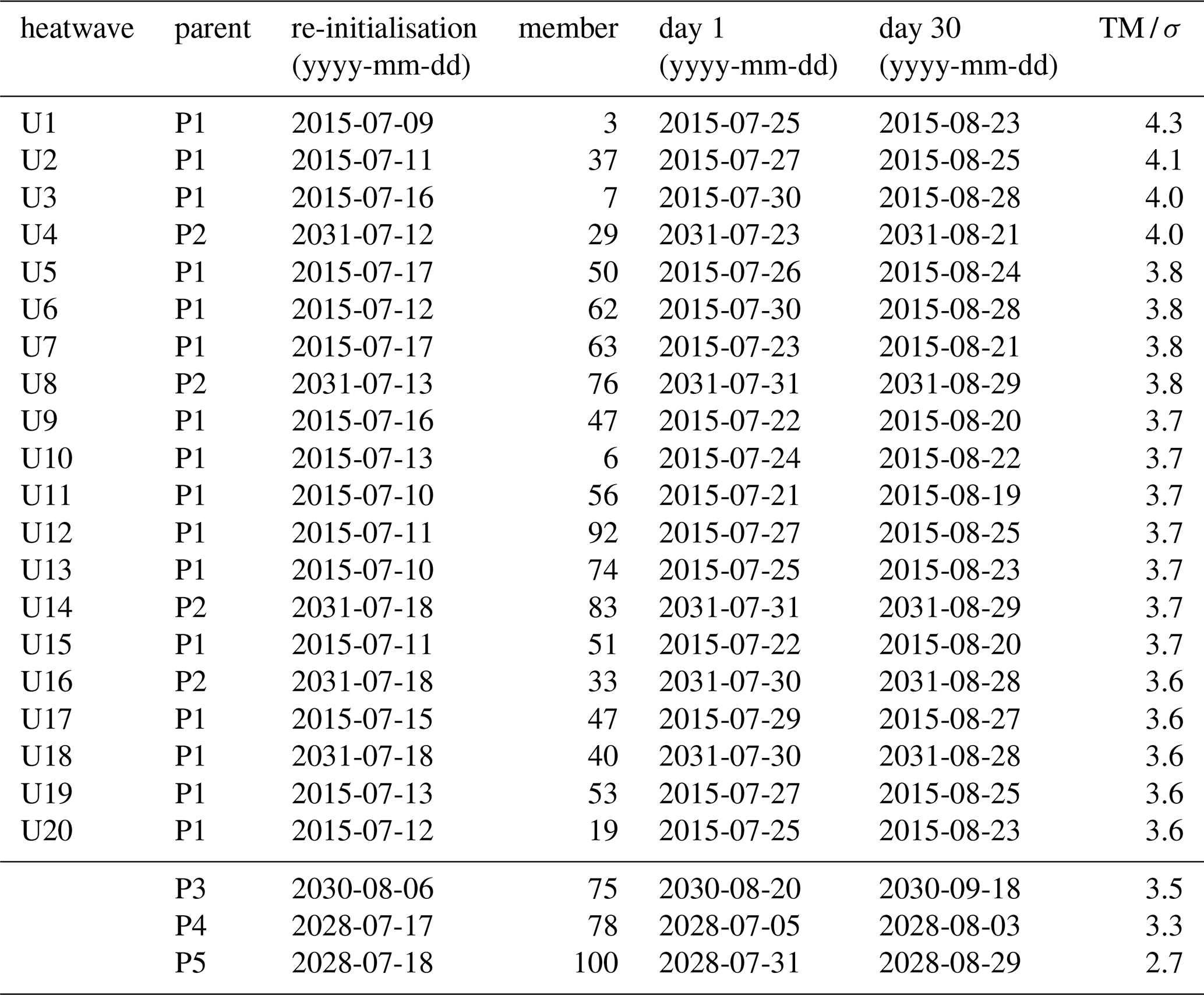
Table B2 Historical 30 d heatwaves in WE selected from ERA5 (beginning and end of the selected 30 d period), sorted in descending order by their 30 d mean TM anomaly.

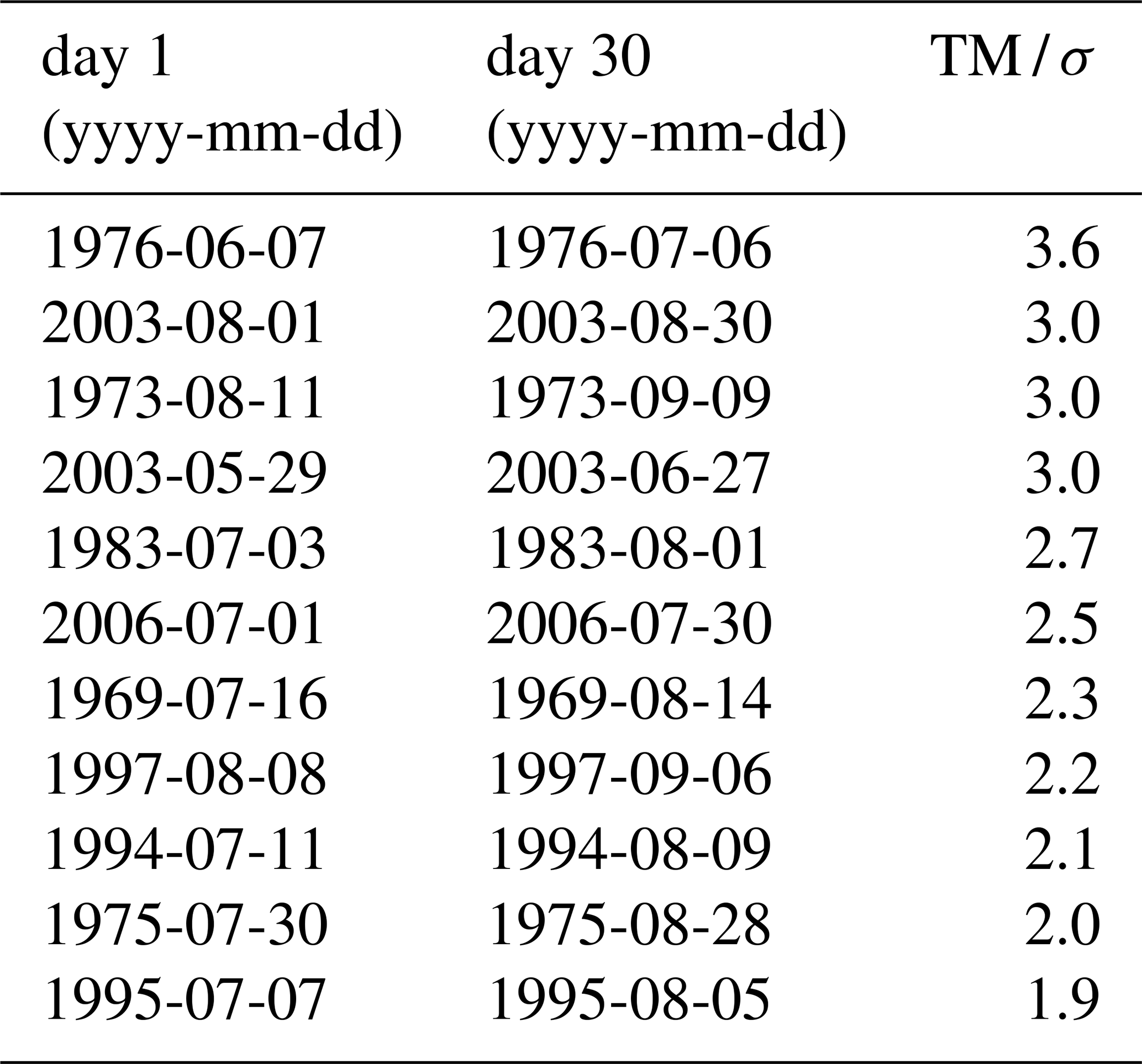
Table B3 Recent 30 d heatwaves in WE selected from ERA5 (beginning and end of the selected 30 d period) in chronological order, with their absolute 30 d mean TM.

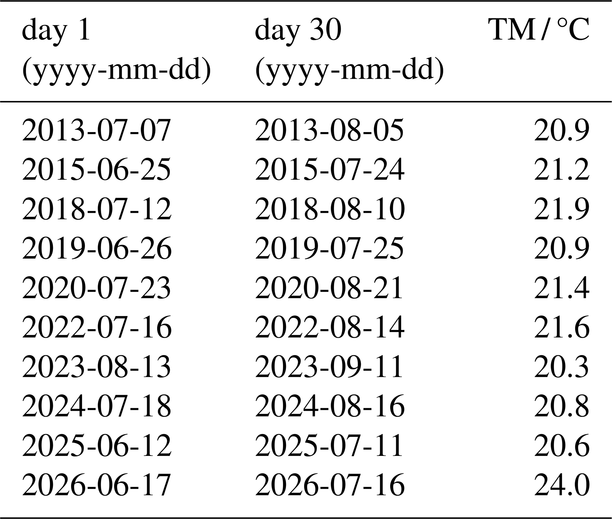
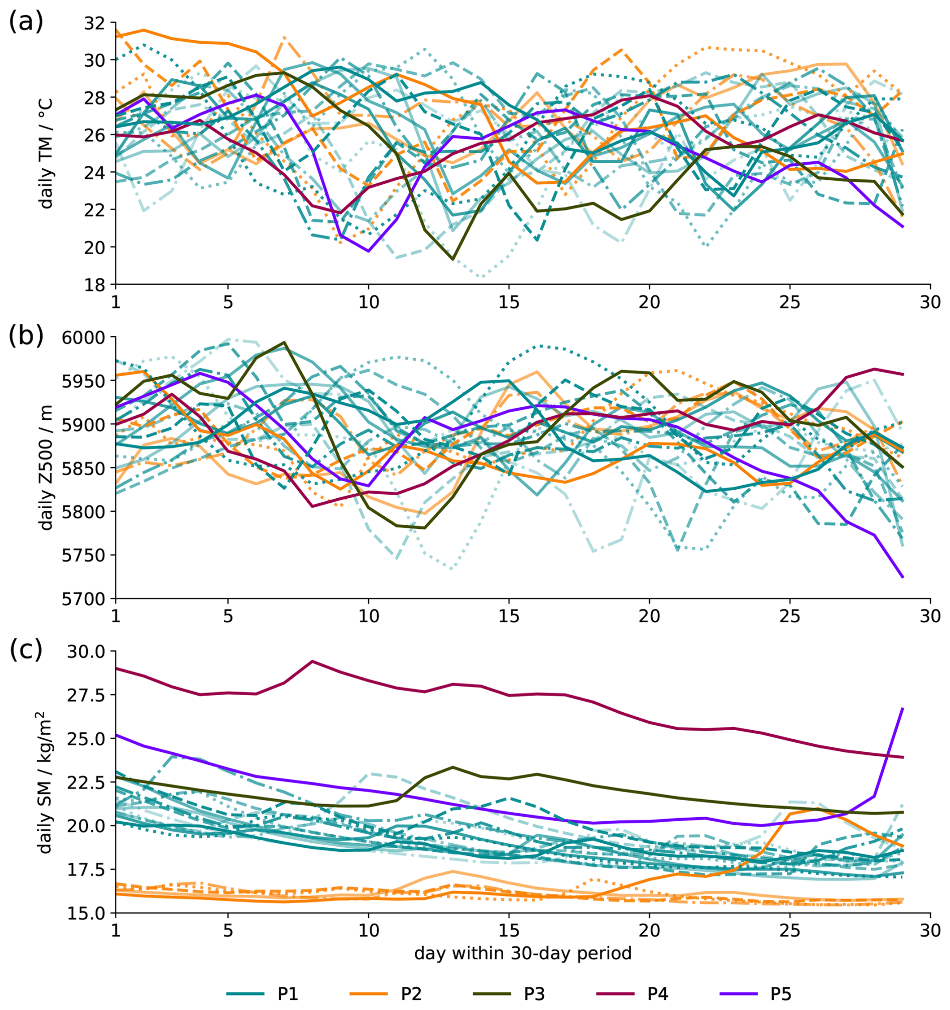
Figure B1 Daily values of (a) TM, (b) Z500, (c) SM during the unprecedented heatwaves (P1, P2) and precedented heatwaves (P3–P5).

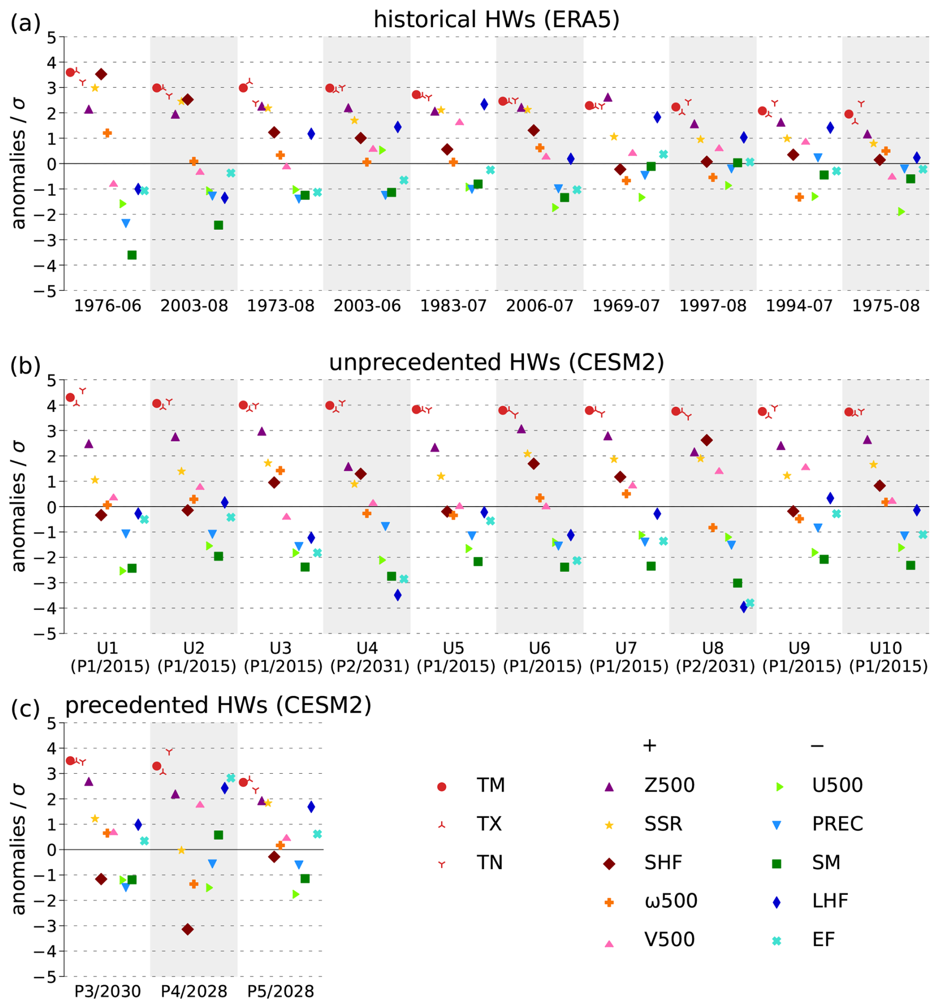
Figure B2 Anomalies of heatwave characteristics and drivers in WE of selected heatwaves (Table C). (a) Ten most extreme historical month-long heatwaves in ERA5 (Table B2) (b) Ten most extreme unprecedented month-long heatwaves in CESM2 ensemble boosting simulations (Table B1). (c) The most extreme heatwaves from the parent ensembles P3–P5 (Table B1). Shown are the temperature variables (red), and variables with expected positive (“+”) and negative (“−”) anomalies during heatwaves. This separation is a simplification primarily adopted for ease of visualization; several variables feature substantial anomalies of both signs during heatwaves.

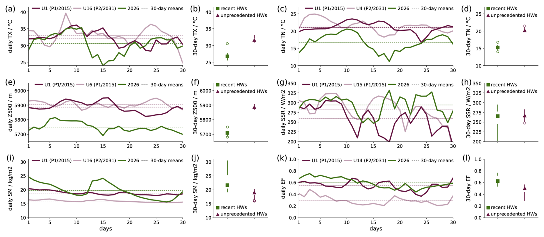
Figure B3 Absolute values in selected variables of unprecedented heatwaves and recent heatwaves. Time series for the 2026 heatwave (green) and for two unprecedented heatwaves: the most extreme in terms of TM anomaly (U1), and the most extreme in terms of absolute value of the respective variable (first and third column). 30 d means of unprecedented and recent heatwaves: Median (filled symbols), inter-quartile range (IQR, empty space), whiskers (1.5 IQR, solid lines) and outliers (empty circles) (second and fourth column).

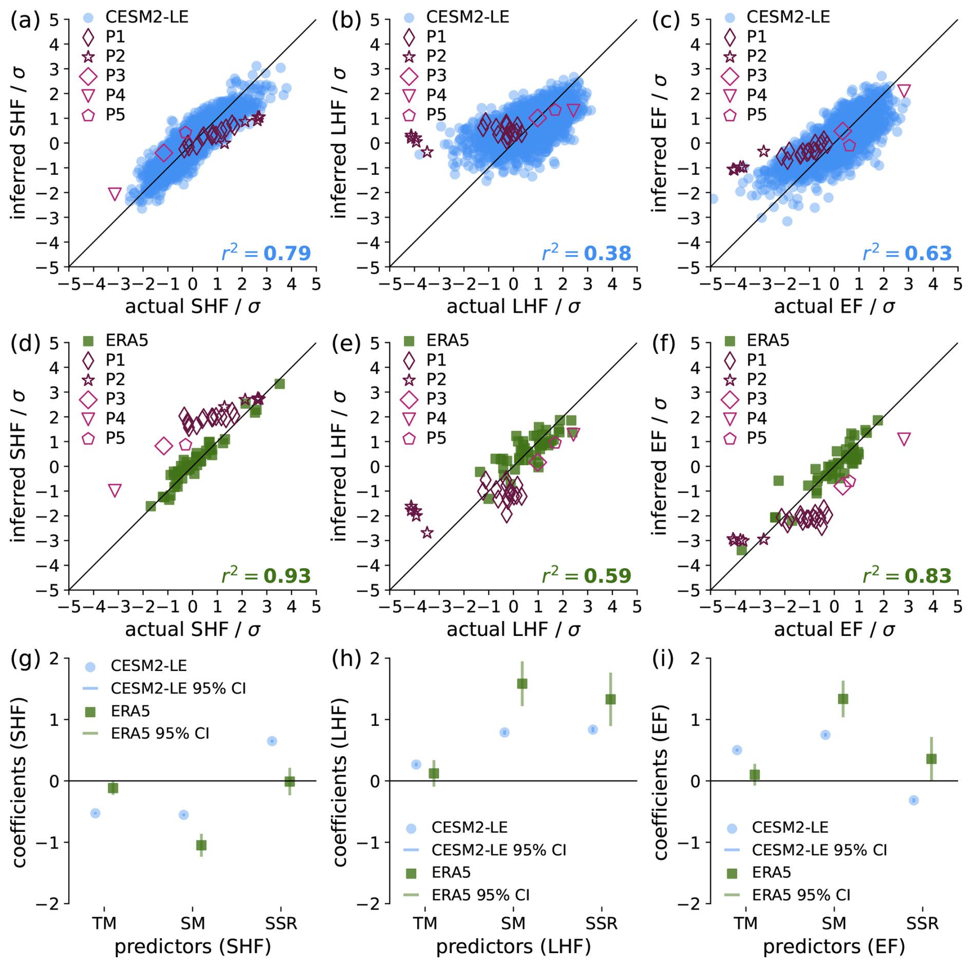
Figure B4 Actual anomalies of SHF (a, d), LHF (b, e), and EF (c, f) and anomalies inferred using our multilinear statistical model. Shown are the training data, namely the annual maxima of 30 d TM anomalies in WE during the summer season (JJA) in CESM2-LE (a–c, blue circles) and in ERA5 (d–f, green squares), respectively. The model is applied to 30 d anomalies of SHF, LHF, and EF in WE during the unprecedented heatwaves (purple) and three less extreme heatwaves from CESM2 boosting simulations (pink). For reference, the 1:1 line and the explained variance r² of each model are also shown. The regression coefficients of each predictor and their 95 % confidence intervals (CI) are compared for LHF (g), SHF (h), and EF (i).

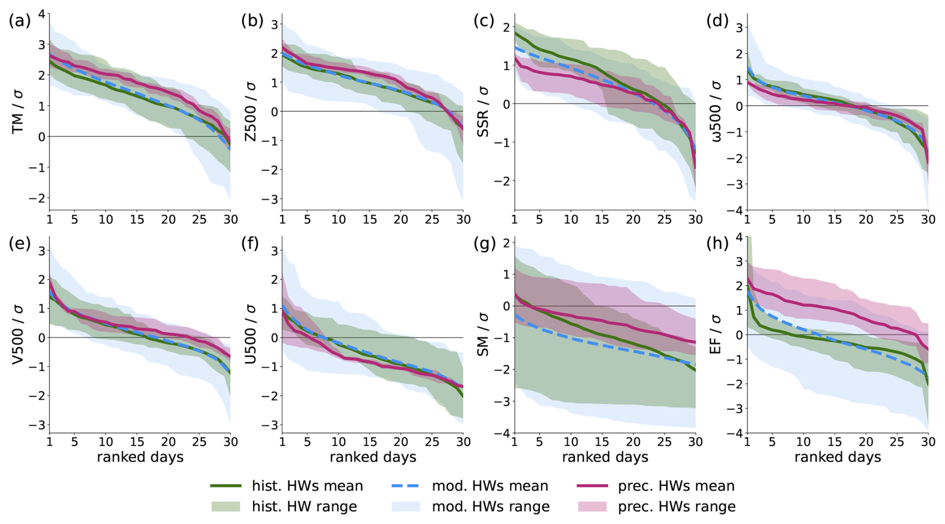
Figure B5 Ranked daily anomalies of heatwave characteristics and drivers during historical heatwaves (green), moderate heatwaves (blue), and precedented heatwaves from CESM2 boosting simulations (pin). Variables are sorted from highest to lowest anomalies, meaning that the most favourable conditions for heatwaves can be found at low ranked days panels (a)–(e), but at high ranked days for panels (f)–(h).

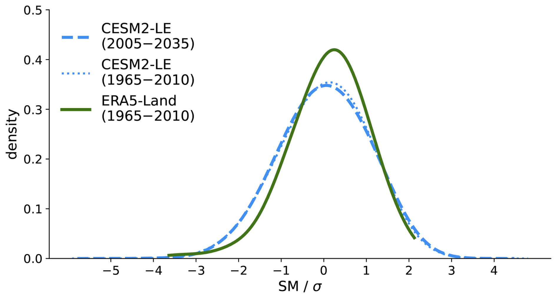
Figure B6 Kernel density estimates of 30 d SM anomalies during the summer season (JJA) in ERA5-Land (1965–2010, green) and in CESM2-LE (1965–2010 and 2005–2035, blue), using a Gaussian kernel with a bandwidth of 0.5 σ, truncated at the data limits.

Appendix C: Heatwave characteristics and drivers analysed in this study

TM	daily mean temperature
TX	daily maximum temperature
TN	daily minimum temperature
DTR	diurnal temperature range
Z500	500 hPa geopotential height
U500	500 hPa zonal wind (positive eastwards)
V500	500 hPa meridional wind (positive northwards)
ω500	500 hPa vertical wind (positive downwards)
SSR	surface downwelling solar flux (positive downwards)
PREC	total precipitation
SM	top-layer soil moisture
LHF	surface latent heat flux (positive upwards)
SHF	surface sensible heat flux (positive upwards)
EF	surface evaporative fraction