The role of atmospheric circulation changes in Western European warm season heat extremes

Climate change has led to an intensification of summer heat extremes, with especially pronounced warming over Western Europe. Here, the maximum and mean of the daily maximum summer temperatures have warmed 3.3 [2.5–4.2] and 2.4 [1.8–3.1] times faster than global mean temperatures. A large part of this enhanced warming can be attributed to dynamical changes. The effects of climate change on springtime heat extremes and circulation changes are less well understood, though changes in spring can influence summer via soil moisture memory. Here we show that between 1950 and 2023, the maximum and mean of the daily maximum spring temperatures in Western Europe have intensified 2.2 [1.2–3.2] and 2.0 [1.3–2.6] times faster than global warming respectively. We show that most of this enhanced warming can be attributed to thermodynamical effects. However, using circulation analogues, we show that locally more than a third of the total temperature trends can be attributed to changes in atmospheric circulation. Our findings suggest that southerly flow patterns, characterized by high pressure over Western Europe and low pressure over the Eastern Atlantic, might become more frequent and intense in spring, which could contribute to the warming trend. Finally, individual ensemble members from large ensemble historical climate model simulations show that those models are capable of simulating temperature trends nearly as extreme as observed, but the model mean underestimates the Western European trends. Future research could expand on this study by further analysing whether the observed dynamical trends are forced or due to natural variability.

1 Introduction

Human-induced climate change has led to the intensification of heat extremes, and their impacts are expected to increase even more with global warming in the future (IPCC, 2021). Extreme heat can deteriorate health (Kjellstrom et al., 2010), cause excess mortality (Yang et al., 2021), affect ecosystems, and threaten food security (Horton et al., 2016). Moreover, extreme heat can cause additional economic damages through reduced productivity, with some heatwave events in Europe causing losses of up to 0.5 % of the European gross domestic product (García-León et al., 2021).

Although most land areas have experienced an increase in heat extremes, some regions are warming faster than others. Globally, the strongest warming of the hottest days is expected to be around 1.5 to 2 times the rate of global-mean, annual-mean warming (IPCC, 2021). However, Vautard et al. (2023) show that summer heat extremes for Western Europe are warming much faster, up to 5 times faster than the global mean temperature trend. Other studies also find rapid warming trends for European summers and identify Europe as a hotspot for heatwaves (Dong and Sutton, 2025; Rousi et al., 2022).

Such trends in extremes can partly be attributed to thermodynamical effects, e.g. warming caused by increased atmospheric greenhouse gas concentrations, enhanced warming over land as compared to oceans, and increased evaporation contributing to soil moisture depletion. However, although these processes are typically less well understood, trends in extremes can also partly be explained by atmospheric dynamical changes (IPCC, 2021; Rousi et al., 2022; Shaw et al., 2024; Singh et al., 2023). Vautard et al. (2023) focus on “Southerly Flow” (SF) patterns, whose increase in both frequency and persistence is the main driver of the dynamical component of the summer heat extreme trends. These patterns contain an anticyclonic component over Central Europe and are characterized by the transport of warm air from more southern regions towards Western Europe. This can lead to extreme temperatures, as seen during the heatwaves in June and July 2019, when advection of air from North Africa, caused by subtropical ridges, resulted in temperatures of 46 °C in France and other record-breaking temperatures in the Netherlands, Belgium, and Germany (Sousa et al., 2020; Vautard et al., 2020). One specific day of the June 2019 heatwave, the SF event on 29 June 2019, will be used later in this study to analyse changes in similar SF days.

Climate models underestimate trends in heat extremes for Western Europe, especially the trend in the maximum of the daily maximum summer temperatures (Vautard et al., 2023). Models also underestimate the increase in frequency of SF days and the dynamical contribution to the temperature trends, which explains a large part of the mismatch (Vautard et al., 2023). Similar underestimations of Western European heat extremes by climate models are found in other studies (e.g., Kornhuber et al., 2024; Lorenz et al., 2019; Patterson, 2023). Climate models play an essential role in understanding future changes, regional climate impact assessments, and weighing possible adaptation and mitigation strategies (e.g., IPCC, 2023; Lopez et al., 2009). Therefore, it is important to analyse the performance and limitations of these models and understand what causes the differences between simulations and observations.

One factor that can influence summer heat extremes is the springtime soil moisture (e.g., Whan et al., 2015). Soil moisture deficits in spring can persist into the summer, where they can influence heat extremes by limiting the latent heat flux, thereby increasing the amount of energy that is available for the sensible heat flux (Seneviratne et al., 2010; Wu and Zhang, 2015). Spring temperatures, in turn, can influence spring soil moisture in different ways. Extremely warm springs can lead to an earlier start of the growing season, resulting in prolonged evapotranspiration and reduced soil moisture (Fischer et al., 2007; Liu and Zhang, 2020). Warmer springs can also lead to a higher evaporative demand, potentially leading to more evapotranspiration and decreased soil moisture (Seneviratne et al., 2010). However, spring heat extremes are less studied compared to summer heat extremes (Sulikowska and Wypych, 2021).

To better understand how these processes, and their influence on summer heat extremes, might have changed due to global warming, this study investigates spring heat extremes in Western Europe. We analyse how fast Western European spring heat extremes are intensifying and what part of this intensification can be attributed to atmospheric dynamical changes. Since the analysis of spring heat extremes in this study applies a similar approach as used by Vautard et al. (2023), their findings on summer heat extremes will be reproduced as well to validate the results. Moreover, it is investigated how Southerly Flow patterns over Western Europe have changed in spring and how they are distributed over the longer warm season. Finally, we analyse how climate models perform in reproducing this seasonal behaviour and long-term trends.

2 Data and methods

2.1 Total temperature trends and dynamical contributions

Trends in spring, March–April–May (MAM), and summer, June–July–August (JJA), heat extremes have been calculated for the period 1950–2023, using the European Centre for Medium-Range Weather Forecasts (ECMWF) ERA5 reanalysis dataset (Hersbach et al., 2020). The intensification of the maximum (TXx) and the mean (TXm) of the daily maximum temperatures in a season are compared to the rate of global warming, expressed in degrees Celsius of warming per global warming degree (°C per GWD), using the method applied in Vautard et al. (2023). Part of these trends can be explained by changes in atmospheric circulation patterns. For example, more occurrences of circulation patterns associated with warm weather can increase temperatures, even without the thermodynamical effects of global warming. To isolate this dynamical contribution and remove the thermodynamical component, trends have also been calculated from a temperature time series in which all temperatures have been scaled to an arbitrary reference warming level, using 2023 as a reference year, and in which temperature fields have been replaced by the fields of days with a similar circulation pattern. Details on the calculation of the trends, the thermodynamical correction, and the “shuffling” of the temperature time series are described in Vautard et al. (2023). For both the total and dynamical temperature trends, a Wald test is used to determine whether the trend at a location is significantly different from 0. The average trends for Western Europe are calculated as the trends in the area-weighted averages of the TXx and TXm values over the land areas within 5° W to 15° E and 45 to 55° N (Fig. 1, box B). A land mask was derived from the E-OBS dataset (Cornes et al., 2018). A 95 % confidence interval for the average trends has been calculated as 1.96 times the standard error of the slope, and is shown in square brackets after the trend estimates.

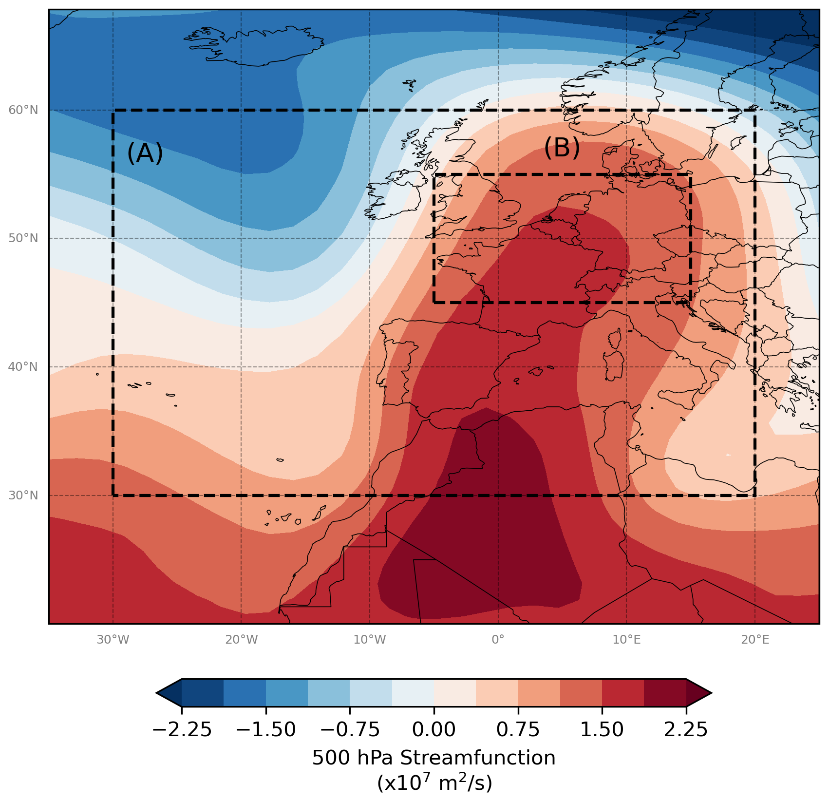
Figure 1 The 500 hPa streamfunction for the Southerly Flow event on 29 June 2019. Box (A) shows the domain used to select analogues. Box (B) shows the area over which trends for Western Europe are averaged.

2.2 Circulation analogues

To analyse the dynamical component of the temperature trends and the changes in SF patterns, circulation analogues have been used. An analogue is a day that has a similar atmospheric circulation as a given event, which for example allows for the analyses of temperatures conditioned to different circulation patterns (Jézéquel et al., 2018). In this study, analogue days were selected based on their 500 hPa streamfunction within 30° W to 20° E and 30 to 60° N (Fig. 1, box A), as in Vautard et al. (2023). To select the best analogues, the Euclidean distance (ED) between the streamfunction fields of a selected event and each day in the season of interest is calculated as described in Thompson et al. (2024a). A lower ED indicates a better analogue, but the event itself (ED = 0) cannot be its own analogue. Moreover, analogues have to be separated by at least 6 d to prevent selecting more analogues from events that have already been selected. To ensure the analogue selection is focused on the actual circulation pattern, rather than absolute streamfunction values, all daily streamfunction fields were prepared by subtracting the spatial mean of all streamfunction values within the domain from each individual value within the domain. This preserves the gradients, and thus the wind field pattern as described by the contour lines, whilst removing any differences in absolute values.

2.3 Southerly Flow patterns

To analyse whether and how SF patterns occurring in spring have changed over time, different characteristics of the analogues for a selected event have been investigated using the ERA5 reanalysis dataset. Figure 1 shows the 500 hPa streamfunction field for the selected SF event on 29 June 2019. This event was part of the hottest June on record for Europe and its circulation pattern is the most representative of days on which the maximum summer temperature is recorded in central France (Vautard et al., 2020, 2023).

The first methods to assess changes in SF patterns analyse differences between analogue sets from two 30-year periods. From both the past period (1950–1979) and the present period (1994–2023), the 30 spring days with circulation patterns closest to the selected SF event are selected as analogues. Between these two periods, changes in typicality, persistence, and intensity have been analysed using the same methods as described in Thompson et al. (2024a). The typicality of the event (t_event) within a period is defined as the inverse of the sum of the 30 EDs associated with the selected analogues. The typicality of each selected analogue (t_analogue) is assessed in the same way, by finding its best analogues and using their EDs. The typicality can also be used as a quality check for the analogues. If the t_event value falls below the distribution of the t_analogue values, this suggests that the analogues are more like the other analogues than like the event itself. This would mean the event is too unique and therefore, the dynamical changes associated with the event cannot be analysed using the analogues (Thompson et al., 2024a).

The persistence of the event (p_event) is defined as the event day itself, plus the number of consecutive days surrounding the event that have a Pearson correlation coefficient with the event of at least 0.9. The correlation coefficient has been calculated using the streamfunction fields over the same domain in which analogue days are selected. The same is calculated for each selected analogue (p_analogue). To test whether the means of the distributions of the t_analogue and p_analogue values differ significantly between the two time periods, a t-test is performed. The significance of changes in intensity, defined as the difference between the means of the streamfunction fields from the 30 selected analogues for both periods, is also assessed for each location using a t-test.

To test whether the SF analogues are also changing when using a different method, the similarity approach as used by Thompson et al. (2024b) has been adapted. Rather than using the 30 best analogues over an entire period, the best analogue day within each year is selected. The similarity for a year is then given by 1 minus the ratio of the selected analogue's ED to the ED of the worst analogue day from both periods combined. This method has been applied to the same 30-year periods, and a t-test was performed to analyse the statistical difference between the means of the values from both periods.

As a final method to assess changes in SF patterns, the frequency of SF patterns and how their occurrences are distributed over a longer warm season (MAMJJAS) have been analysed. To achieve this, an ED threshold is used instead of a fixed number of analogues in a season. This time, the entire dataset is divided into a past (1950–1986) and a present (1987–2023) period. For each month in the warm season, the number of analogues with an ED below a certain threshold in that period is counted. The threshold is the same for all months and is taken as the fifth percentile of all EDs in the analysed months of both periods combined. The streamfunction field corresponding to the threshold is shown in the Supplement (Fig. S1). To test whether changes in frequency are statistically significant, the trend in the number of analogues per year over both periods combined is calculated for each month. A Wald test is then used to determine whether a trend is significantly different from 0.

2.4 Climate models

To analyse the ability of climate models to simulate the observed temperature trends and changes in SF days, part of the analysis has been repeated with climate model output data from the Large Ensemble Single Forcing Model Intercomparison Project (LESFMIP) (Smith et al., 2022). This was done using two global climate models that are also part of the Coupled Model Intercomparison Project Phase 6 (CMIP6), the HadGEM3 and MIROC6 models. These models were chosen due to the high number of ensembles available at the time of analysis. For the HadGEM3 model, more details on the exact simulation that was used (HadGEM3-GC31-LL) and specifics of the model are described in Andrews et al. (2020) and Ridley et al. (2019). For the MIROC6 model, more information on the simulation, model components, and their resolution is described by Shiogama et al. (2023) and Tatebe et al. (2019). Although global climate models are, for example, known to underestimate the frequency of blocking events, a weather pattern often related to summer heat extremes, the newer CMIP6 models do already generally perform better than older model versions (Davini and D'Andrea, 2020; Schiemann et al., 2020). Palmer et al. (2023) show that the MIROC6 model's performance in terms of summer blocking frequency for Europe is sufficient (satisfactory on a scale with satisfactory, unsatisfactory and inadequate). The HadGEM3 model's performance regarding summer blocking frequency is labelled unsatisfactory, but the model does perform particularly well in capturing the large-scale circulation patterns over Europe for both summer and winter (Palmer et al., 2023). Both models have also been used before in studies investigating European summer temperature trends (e.g., Patterson, 2023) and dynamical contributions to these trends (e.g., Vautard et al., 2023).

To compare the ERA5 and model results, the data have been regridded to the HadGEM3 model resolution (1.875° × 1.25°). When calculating the mean trend over Western Europe with the regridded data, only cells that consist entirely of land are considered. From both models, data covering the 1950–2014 period from the historical-forcing runs were used. Therefore, the ERA5 analyses have also been repeated with the 1950–2014 period to make comparisons possible. For the total temperature trends, the analysis has been repeated using 55 ensemble members from the HadGEM3 model and 50 ensemble members from the MIROC6 model. Due to missing data in the daily wind fields from the models, the analogue analyses that use streamfunction have only been repeated with five ensemble members from the HadGEM3 model and three ensemble members from the MIROC6 model. These eight ensemble members have been used to repeat the analysis of the dynamical component of the temperature trend and the typicality, persistence, and intensity of SF days. For the analyses investigating SF days using the model data, the past period remains 1950–1979 and the present period becomes 1985–2014. Ensemble members are treated independently in all steps of the repeated analyses.

3 Results

3.1 Total temperature trends and the dynamical contributions

Figure 2 shows the total trends in spring and summer temperature extremes, as well as the dynamical contributions to these trends, from the ERA5 dataset. For spring, the largest TXx trends are found in Norway and Spain, with trends in Norway reaching more than 7 °C per GWD (Fig. 2A). For Western Europe, the warming is somewhat slower, but still significantly faster than global warming with an average spring TXx trend for land areas equalling 2.2 °C per GWD [1.2–3.2 °C per GWD] and maximum trends of more than 3 °C per GWD around the north of Italy. The total spring TXm trend is found to have smaller regional differences with generally lower trends as well (Fig. 2C). The maximum trends reach up to 2.5 °C per GWD and are found in for example Spain and Sweden. For Western Europe, the average spring TXm trend is 2.0 °C per GWD [1.3–2.6 °C per GWD]. Both the total TXx and TXm trends are found to be significant on a 95 % confidence level for most of Europe.

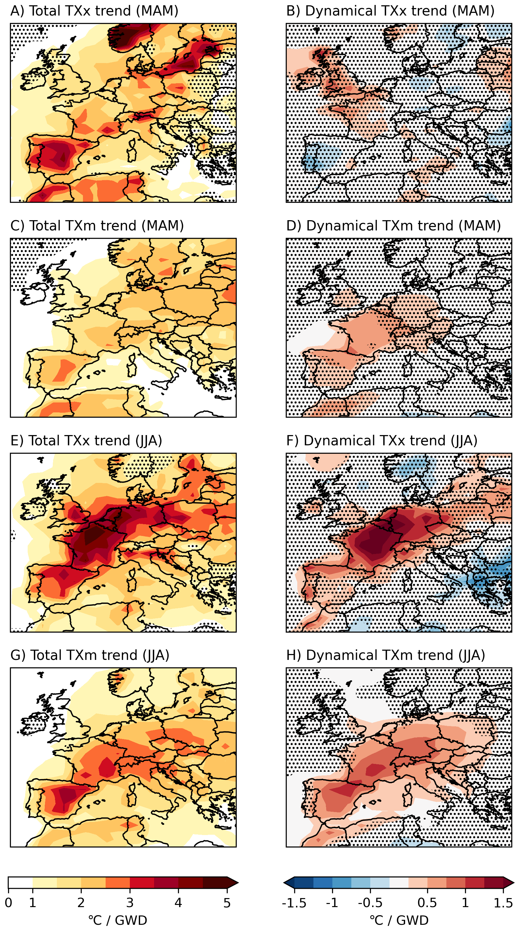
Figure 2 The total trends in the maximum (TXx) and the mean (TXm) of the daily maximum temperatures in a season, for spring and summer, and the dynamical contributions to these trends. Trends are calculated using the ERA5 dataset and are expressed in the amount of warming, in degrees Celsius, per global warming degree (GWD). Dotted areas represent regions where the trend is not significant on a 95 % confidence level.

For the dynamical spring TXx trend, values of around −1 to 1 °C per GWD are found (Fig. 2B). For Western Europe, this results in an average dynamical contribution to the TXx trend of 0.2 °C per GWD [−0.3–0.6 °C per GWD]. However, note that most of these trends are insignificant on a 95 % confidence level, apart from the warming in some small regions like the south of the United Kingdom and Italy, the west of France, and the east of Spain. A small area in the east of Romania is the only region with a significant cooling trend. The dynamical contribution to the spring TXm trend is a warming over all of Western Europe, with an average trend of 0.4 °C per GWD [−0.1–1.0 °C per GWD] and significant trends between 0.5 and 1 °C per GWD over parts of France and Spain (Fig. 2D). Note that, since European temperatures typically increase throughout spring, the spring TXx trend could be biased towards May rather than equally representing the entire season. However, by repeating the analyses with anomalies from the daily climatological mean temperature instead of absolute temperatures, it has been shown that this has little influence on the results, as shown in Fig. S2.

For summer, the largest TXx trends are found in Western Europe, with a maximum of more than 5 °C per GWD and an average Western European trend of 3.3 °C per GWD [2.5–4.2 °C per GWD] (Fig. 2E). The dynamical contributions to the TXx trends are largest in Western Europe as well, with an average of 1.0 °C per GWD [0.5–1.5 °C per GWD] (Fig. 2F). In contrast, summer TXm trends are overall lower, with a Western European average of 2.4 °C per GWD [1.8–3.1 °C per GWD] and an average dynamical contribution of 0.7 °C per GWD [0.3–1.1 °C per GWD] (Fig. 2G and H). In general, both the spatial pattern and the magnitude of the summer trends are similar to the trends up to 2022 as found by Vautard et al. (2023). To give an indication of the effect of using a stricter statistical test, Fig. S3 shows the same results, but applying the Benjamini-Hochberg procedure to control the false discovery rate as described in Wilks (2016). This mainly affects the significance of the dynamical spring trends, for which all trends become statistically insignificant when applying this stricter test.

3.2 Changes in Southerly Flow days

To assess the changes in frequency and persistence of SF events, we analyse the difference in typicality and persistence between the past and present time periods for the selected SF event (Fig. 3). For both periods, the t_event falls within the distribution of the t_analogue values, showing the 30 analogues are of sufficient quality to investigate dynamical changes associated with the event (Fig. 3A). The typicality of the event in the present period is higher compared to the past period, showing that the closest analogues in the present period are more similar to the event. This likely represents an increase in frequency of similar events – with a likely increase in analogues above a certain threshold, though this is not explicitly shown here. The t_analogue distributions support this finding, the higher mean value in the present period indicates that the analogues, that became more similar to the event, also become more typical to each other. However, note that the difference between the means of the t_analogue distributions is not significant on a 95 % confidence level.

Whereas the event itself only persisted for 1 d, Fig. 3B shows that most of the analogues persist longer, with one analogue from the past period persisting for up to 8 d. Note that, since a persistence of 8 d exceeds the analogue separation range of 6 d, it has been checked that not two analogues were selected from this single event. However, apart from this single analogue, the distributions of the p_analogue values did not change a lot over time. There seems to be a slight shift from analogues persisting for 2 d towards analogues persisting for 3 d, but the means of both distributions are almost identical.

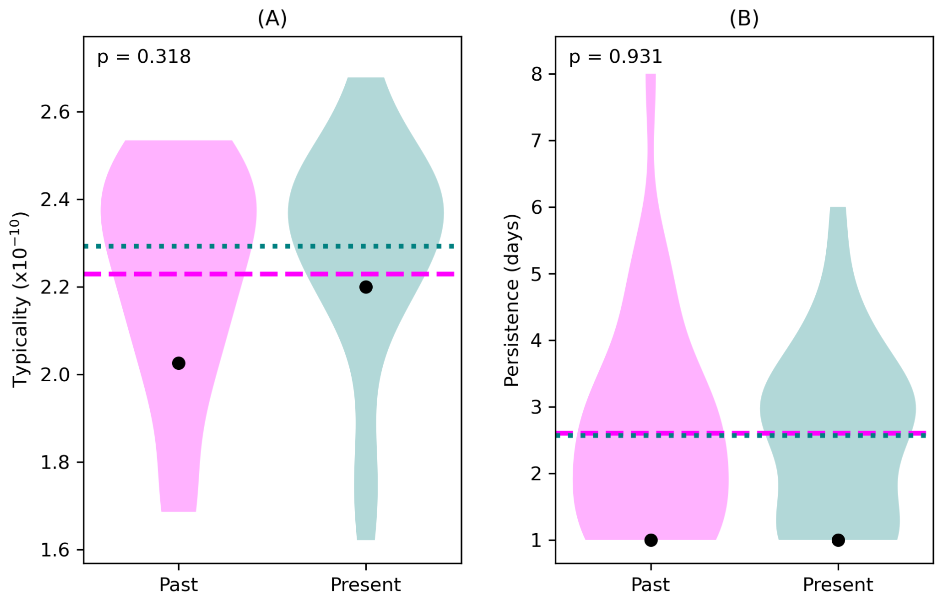
Figure 3 The changes in typicality (A) and persistence (B) for spring between the past (1950–1979) and present (1994–2023) periods. Black dots indicate the typicality and persistence of the event. The violins show the distribution of the t_analogue and p_analogue values, whose means are represented by dashed lines for the past period and dotted lines for the present period. The p-value indicates the statistical significance of the difference between these means.

Figure 4 shows the similarity value for each year in the two time periods. The highest similarity values are found in the present period. Moreover, the mean similarity of the present period is higher compared to the past period, again suggesting that analogues are becoming more similar to the event. However, note that with a p-value of 0.095, the difference between the means is not significant on a 95 % confidence level.

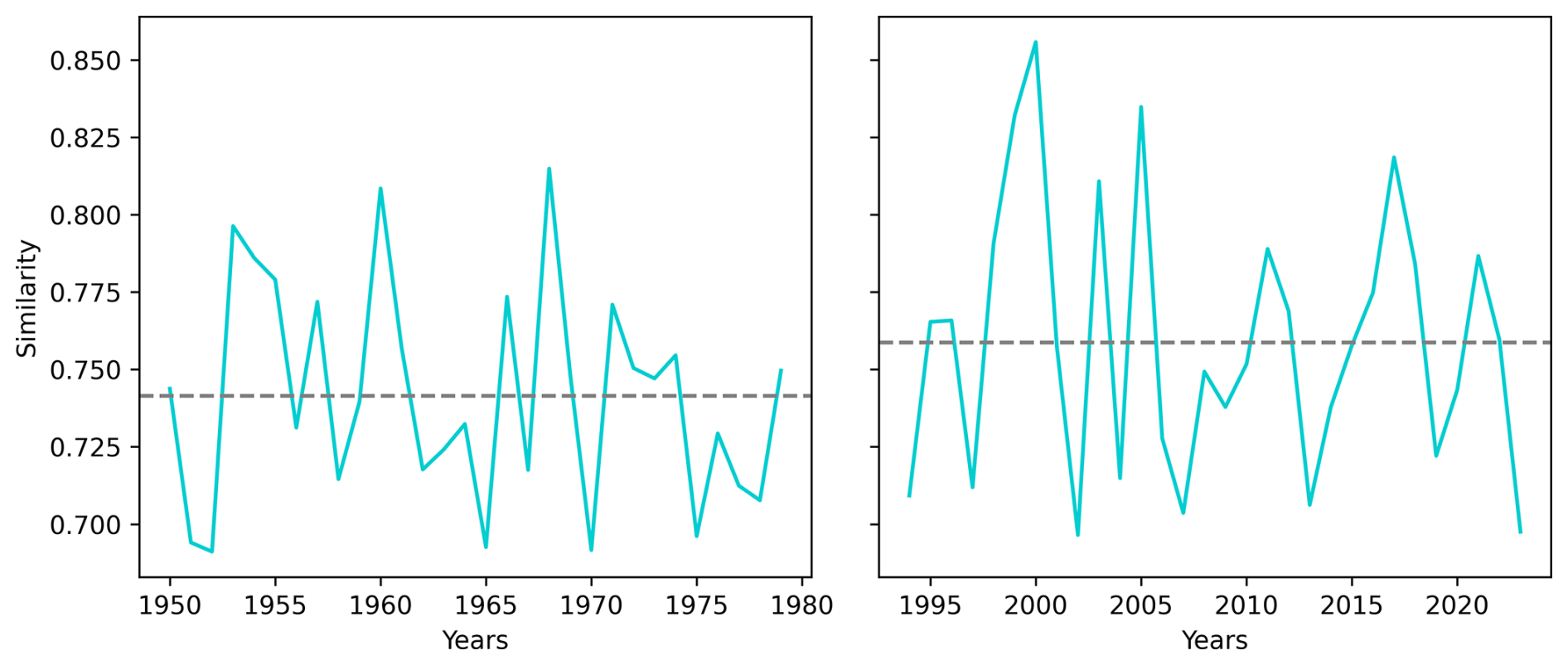
Figure 4 The similarity value of the best analogue in a year, for each year within the past and present time periods. Dashed grey lines represent the mean of all similarity values within a time period.

Figure 5 shows the SF event, the SF analogue composites for both the past and present periods, and the changes in intensity. Over most of Western Europe, there is an increase in streamfunction gradient, indicating a strengthening of the high pressures and a deepening of low pressures. For the higher pressure over Europe, this would result in stronger subsidence of air, and therefore an increase in the intensity of potential heat events. This increase is found to be even stronger, and statistically significant, for parts of France and Spain. Moreover, the increase in streamfunction in the centre of the domain, combined with the decrease in both lower corners of the domain, increases the gradient of the streamfunction. This reflects an increased advection of air from southern regions towards the north, further intensifying the SF days. When comparing the streamfunction pattern from the event with the past composite, the event seems to have higher values over Southern and Western European land, but lower values southeast of Italy and in the southwest corner of the domain. This matches the pattern found in the difference map between the present and past composites, once again confirming that the analogues are becoming more similar to the event over time, as also seen in Fig. 3A, whilst also showing how this happens spatially.

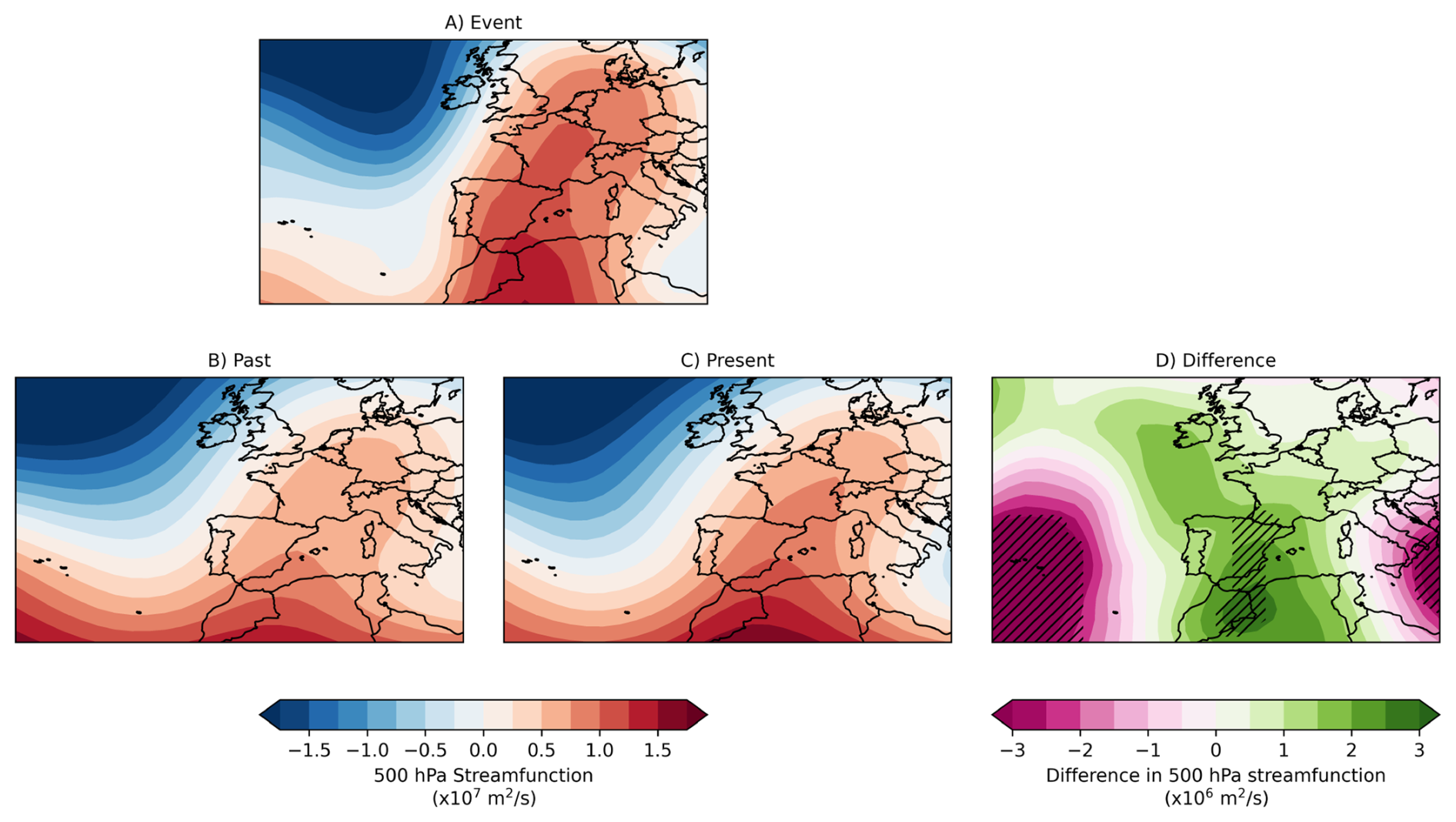
Figure 5 The difference in 500 hPa streamfunction between analogue composites from the present (1994–2023) and past (1950–1979) periods. Hatched areas show regions where the difference is significant on a 95 % confidence level.

Finally, Fig. 6 shows the distribution of SF days over the longer warm season and how their frequency changes over time. It becomes clear that the frequency of SF days in spring has slightly increased over time, but that the increase is much bigger for the summer season. Interestingly, the frequencies in July and September have decreased over time. However, note that June and August are the only analysed months for which the trend in frequency is significantly different from 0 on a 95 % confidence level (Fig. S4). When looking at the distribution over the months, by far the largest amount of SF days occur in summer, especially for the present period. For both time periods, there seems to be a rapid increase in frequency after April.

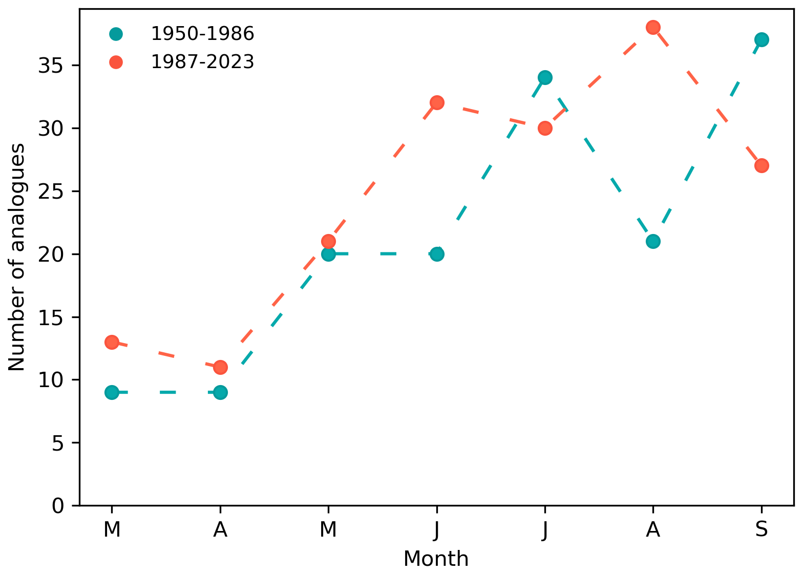
Figure 6 The distribution of analogues within the fifth percentile of Euclidean distances over different months, for two time periods.

3.3 The performance of climate models

To make ERA5 and model results comparable, the total temperature trends have been recalculated using ERA5 data until 2014 (Fig. 7A and B). Although the spatial patterns are comparable to the trends up to 2023, the trends until 2014 actually tend to be larger, with a new maximum of 9 °C per GWD in Norway. Figure 7 also visualizes the performance of the HadGEM3 and MIROC6 models to reproduce these total temperature trends. When looking at the average trends found by the 105 model ensemble members, the models seem to correctly capture the general spatial patterns, with the largest TXx trends found in Norway and Spain and relatively high TXm trends simulated in Eastern Europe (Fig. 7C and D). However, the average modelled trends, especially the TXx trends, are much lower compared to the ERA5 trends with a maximum average TXx trend of 3.4 °C per GWD. The standard deviations of the modelled trends are largest in areas with the highest temperature trends and are especially large for the TXx trends (Fig. 7E and F), indicating that individual ensemble members could reach higher trends. Indeed, the largest TXx trend found in an individual ensemble member equals 8.8 °C per GWD, showing that, although the models on average underestimate the trends, extreme cases as found for ERA5 can be captured by the models. To investigate how many of the individual ensemble members find a large enough trend, Fig. 7G and H show the percentage of ensemble members that find a trend as high as the trend found in ERA5 or higher, for each location. For some areas, like Greece and the south of Italy, most of the ensemble members seem to simulate a large enough trend. However, the trends in most parts of Western Europe are underestimated by more than 70 % of the ensemble members. This is also the case for Spain and parts of Eastern Europe. In general, the TXx trend seems to have the most extreme underestimated trends, like in Norway and the north of Italy. Whereas both the ERA5 TXx and TXm trends are statistically significant over most parts of Europe, the majority of the modelled TXx trends over European land are not (Fig. 7I). For the TXm trend, most ensemble members find statistically significant trends (Fig. 7J).

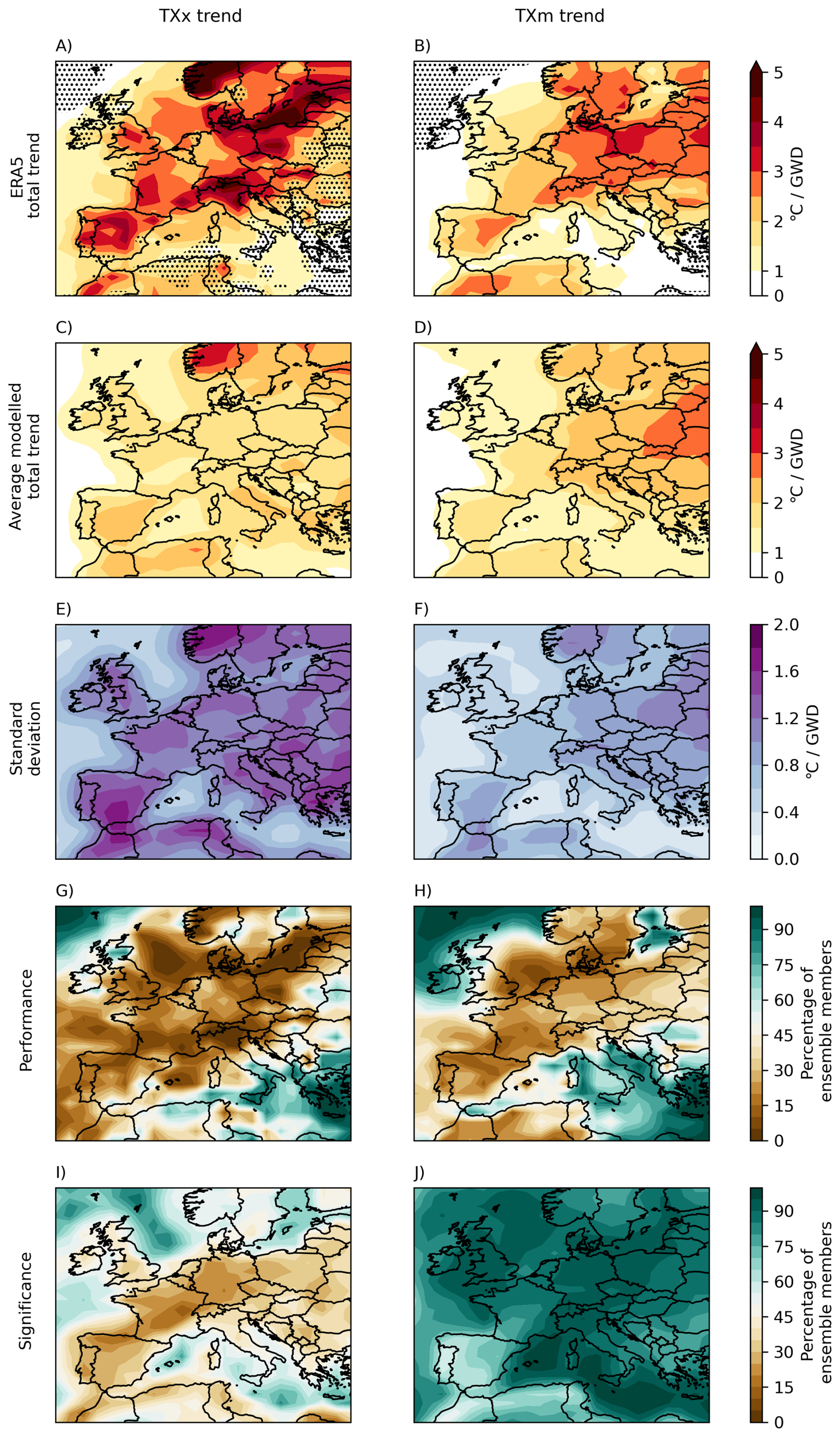
Figure 7 The ERA5 total temperature trends in the maximum (TXx) and the mean (TXm) of the daily maximum spring temperatures up to 2014, the mean trends found by the 105 model ensemble members from the HadGEM3 and MIROC6 models, the standard deviation of the modelled trends, the percentage of the ensemble members that find a trend as high as the ERA5 trend or higher, and the percentage of the ensemble members that find a trend that is statistically significant on a 95 % confidence level.

To further analyse the models' performances for Western Europe, Fig. 8 shows the distribution of the Western European average trends as found by all individual ensemble members. Again, most of the ensemble members underestimate the trend as found in ERA5. For the Western European TXx trend, the mean of the ensemble members equals 1.7 °C per GWD and only 10 out of 105 ensemble members simulate a trend as high as the ERA5 trend. For the TXm trend, the mean is 1.9 °C per GWD and 26 ensemble members find a large enough trend. However, with standard deviations of 0.8 and 0.7 °C per GWD for the TXx and TXm trends respectively, the ERA5 trends of 2.9 and 2.4 °C per GWD do fall within the 95 % confidence interval of the ensemble means. Interestingly, there is a large difference between the two different models. When only taking into account the HadGEM3 model, only one ensemble member finds a TXm trend as high as ERA5, and no ensemble member finds a large enough TXx trend (Fig. S5). With respective TXx and TXm means equalling 1.6 and 1.4 °C per GWD and standard deviations of 0.6 and 0.4 °C per GWD, both the ERA5 trends fall outside of the 95 % confidence interval of the HadGEM3 mean trends.

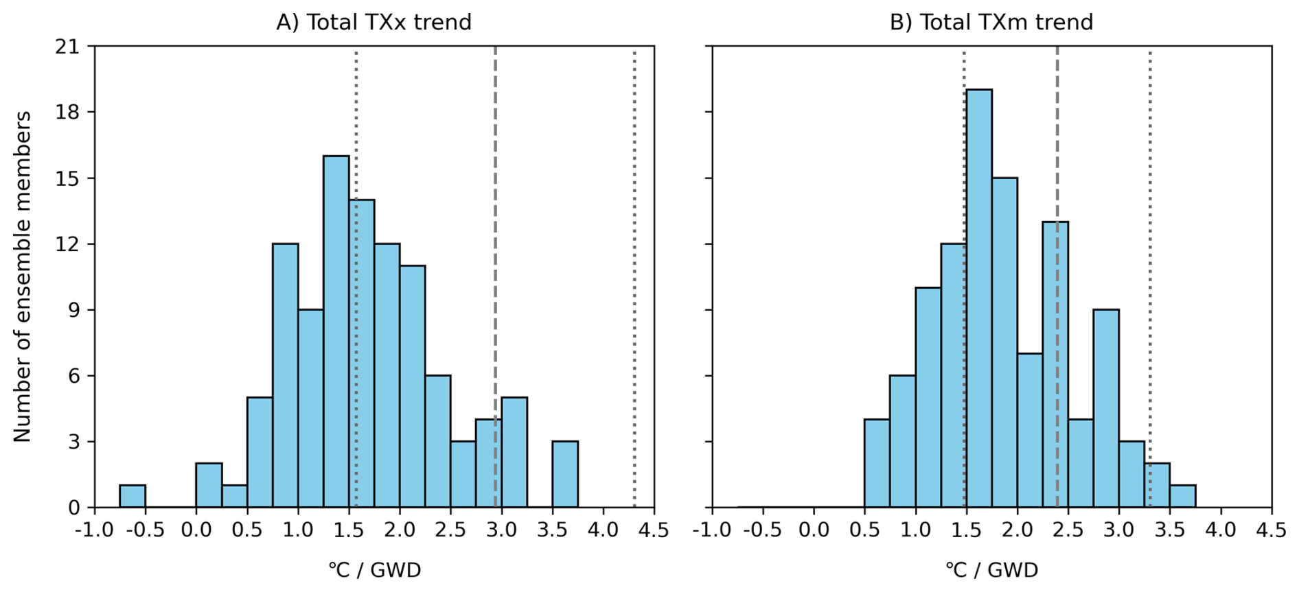
Figure 8 The distribution of the trends in the maximum (TXx) and the mean (TXm) of the daily maximum spring temperatures, averaged for Western Europe, as found by 105 ensemble members from the HadGEM3 and MIROC6 models. The dashed grey lines represent the trends found in ERA5, with dotted lines showing their 95 % confidence interval.

To investigate whether the underestimation of the total temperature trends is caused by an underestimation of the dynamical changes, the analysis of the dynamical trends has been repeated with ERA5 and model data until 2014. The results for the eight ensemble members are shown in the Supplementary Material (Figs. S6 and S7). The result for the TXx trend shows large differences between ensemble members, with half warming and half cooling over Western Europe. All four ensemble members that show a warming find trends larger than observed in ERA5, with maximum trends of 0.73 and 0.86 °C per GWD for the HadGEM3 and MIROC6 models respectively. Therefore, although the average model trend (0.11 °C per GWD) is lower than the observed ERA5 trend (0.26 °C per GWD), the models do not seem to systematically underestimate the dynamical component of the TXx trend. The results for the TXm trend are a little less clear, with an observed ERA5 trend showing a warming over almost all of Europe, and a larger Western European trend compared to the 2023 trend of 0.64 °C per GWD. From the models, only three ensemble members show a warming trend over Western Europe, with a maximum trend of 0.52 °C per GWD, resulting in an average Western European trend of 0.00 °C per GWD. Only one member shows a warming over most of Europe, and three members show a cooling trend over most of Europe.

The typicality and persistence analysis have been repeated for the model ensembles, and the results are shown in Fig. S8. Only two out of the eight ensemble members find an increase in both the t_event and the mean of the t_analogue distribution, and for one of them, the difference between the means is even significant on a 95 % confidence level. However, their increase in the typicality of the event and the absolute typicality values are still lower compared to the typicality found in ERA5. One HadGEM3 ensemble even finds a statistically significant decrease in the mean t_analogue value. There also seems to be a difference between the performance of the models in simulating similar SF days, with each mean of the t_analogue distributions found by the MIROC6 model being similar or higher than the ERA5 means and higher than all means found by the HadGEM3 model. Apart from an analogue persisting up to 10 d, the persistence does not seem to change over time for all ensemble members, who find similar means as found in ERA5.

Finally, the analysis of the intensity of SF days has been repeated, and results are shown in Fig. 9. When looking at the composites of the analogues, all ensemble members still show clear SF patterns. However, the difference between time periods differs a lot between the members. Only one ensemble member shows a pattern similar to ERA5, with an increase in streamfunction magnitude over the north of Africa, Spain, and France and decreases in both lower corners of the domain. For the remaining ensembles, changes are either small and insignificant or show an opposite change with large decreases over European land.

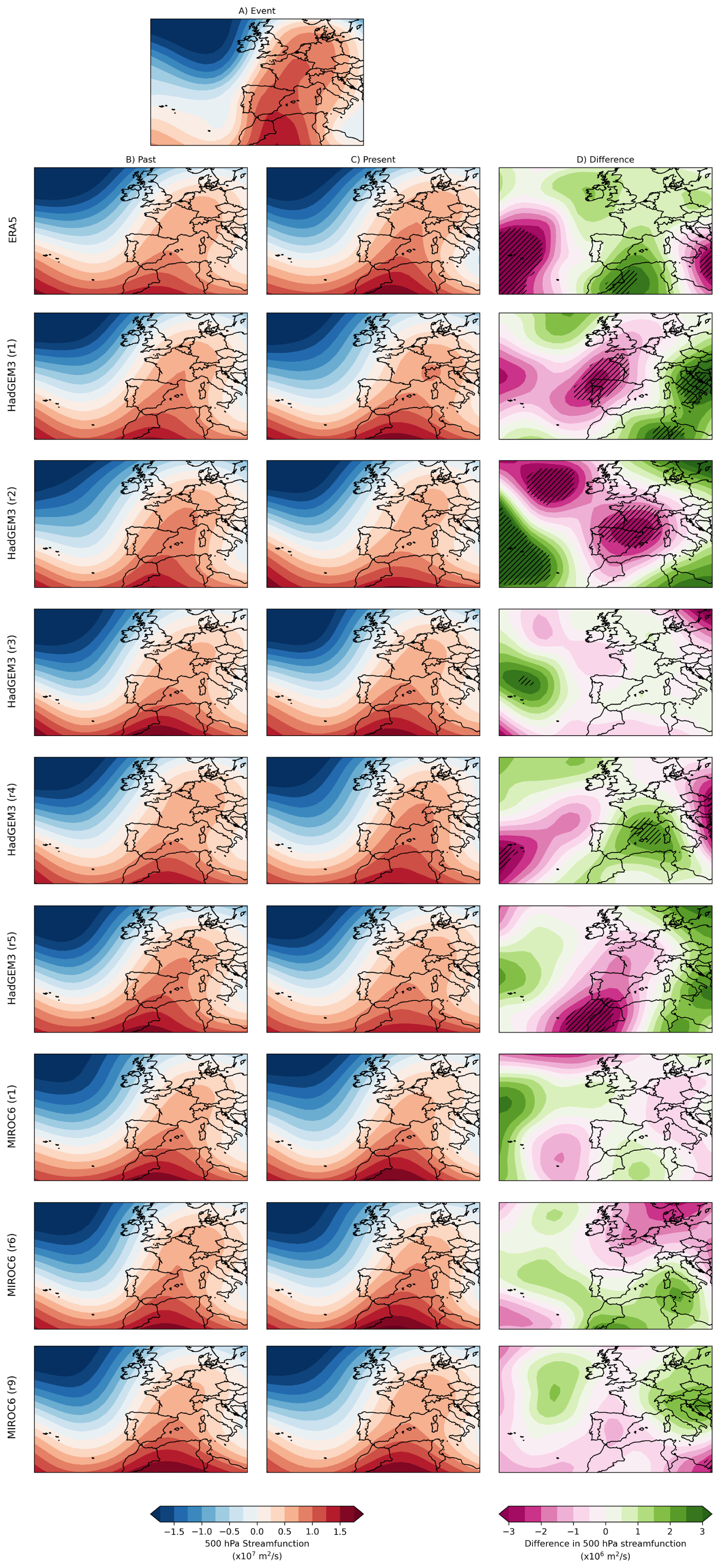
Figure 9 The difference in 500 hPa streamfunction between analogue composites from the past (1950–1979) and present (1985–2014) periods, for ERA5 and the different model ensembles. Hatched areas show regions where the difference is significant on a 95 % confidence level.

4 Discussion

The increase in the typicality of the selected SF event can partly be attributed to a small increase in the frequency of SF days, although the increase in spring is much smaller compared to the increase for the summer season. Vautard et al. (2023) also found a large increase in the frequency of summer SF days. However, they also found an increase in the persistence of these days (24 % between 1950 and 2022), whereas this study shows no clear increase in the persistence of SF days can be detected for springtime. The remaining increase in typicality can be attributed to the fact that SF days are becoming more similar to the selected SF event. With higher pressure over Western European land and a stronger advection of warm air from the south, caused by an increase in the gradient of the streamfunction field, the SF days are becoming more intense. Both changes are part of the dynamical contributions to the total temperature trend and could be important for spring heat extremes. Note that, although the persistence of the analogues may provide some indication of the circulation before or after the analogue days, only using isolated daily streamfunction fields in the analogue selection process does not take into account changes in the large-scale circulation leading up to the selected analogue days. Furthermore, the SF patterns are selected based on streamfunction fields at the mid-troposphere level (Fig. 1), without taking into account the lower-tropospheric circulation, meaning the exact origin and characteristics of surface-level air masses could still vary between analogue days. Finally, instead of 29 June 2019, a different example of an SF event could have been chosen as a reference event, which might have led to different results.

The changes in SF days may partly be caused by changes in land-sea temperature contrast, which is found to be increasing with global warming (e.g., Shaw and Voigt, 2015). A larger temperature contrast also results in a geopotential height contrast. The anticyclonic anomalies over land and cyclonic anomalies over the ocean that can result from this (Kamae et al., 2014), could contribute to the intensification of the Southerly Flow patterns. SF patterns related to heat events over Europe can also be part of a larger Rossby wave (White et al., 2022). For example, several heat extremes over Western Europe were related to a wave 7 pattern, a wave pattern that might also be favoured by a large land-sea temperature contrast in the mid-latitudes (Kornhuber et al., 2019). With an increasing temperature contrast caused by global warming, as well as from spring to summer, this could influence the increases in the frequency of SF days during the warm season and between time periods. Furthermore, it has been hypothesized that a larger land-sea temperature contrast, that can favour a double-jet structure, can amplify such planetary waves as well as lead to more frequent blocking events that influence heat extremes (He et al., 2018; Rousi et al., 2022).

The results show that the Western European spring TXx has warmed with 2.2 °C per GWD. Although not as fast as the summer trend of 3.3 °C per GWD, it is more than twice the rate of global warming. For the TXm trends, there is a smaller difference between seasons, with 2.4 °C per GWD in summer and 2.0 °C per GWD in spring. This rapid spring warming could directly contribute to spring soil moisture deficits and therefore influence the summer extremes in Western Europe.

Other studies have shown that there is a connection between Southern European spring soil moisture deficits and Western European summer heat extremes (e.g., Vautard et al., 2007; Zampieri et al., 2009). Dry soils in Southern Europe result in local warming due to the increase in the sensible heat flux. Moreover, a soil moisture deficit results in drier air as well, which in turn leads to a reduction in cloudiness and therefore amplifies the dry and hot conditions through an increase in radiation. These dry conditions can be propagated towards more northern parts of Europe by southerly winds, where they increase the temperature and evaporative demand, again resulting in drier conditions. Here, the dry soils can influence extreme heat through the previously described feedbacks, as well as by favouring anticyclonic conditions (Vautard et al., 2007; Zampieri et al., 2009). Whereas for summer, the highest TXx trends are found in Western Europe, the highest trends in spring are found in Norway and Spain, the latter of which also has relatively high TXm trends in both spring and summer. Rapid Southern European warming trends in spring, like those found for Spain, could therefore potentially influence Western European summer heat extremes by contributing to the initial soil moisture deficits in Southern Europe needed to start the propagation of drought and heat towards Western Europe.

The most extreme spring trends are found in Norway, with TXx trends of more than 7 °C per GWD. Similar results are found when using different methods to calculate trends, as shown by Sulikowska and Wypych (2021). They find that spring is the season with the largest TXx trend for Western Scandinavia, with an average warming of 0.5 °C per decade between 1950 and 2019. Moreover, they show that when dividing most of Europe into five study domains, and considering all seasons, the Western Scandinavian spring trend is tied for the largest TXx trend with the summer trend in the British Isles domain, covering the Netherlands, Belgium, Ireland, the United Kingdom, and part of France. However, note that the highest trends in Scandinavia found in their study are located in southwestern Finland, an area that shows average trends in this study, and in the north of Finland, an area that is not investigated in this study. Finally, Sulikowska and Wypych (2021) show that the trends in average maximum spring temperatures are higher for Central Europe and Iberia than for the British Isles domain, which seems to match the pattern in the TXm trends found in this study.

The dynamical components of the summer TXx trends are especially high and significant for Western Europe. For spring on the other hand, there are lower and mostly insignificant dynamical components over Western Europe, with even a cooling trend over parts of Germany. However, there are still some small regions in Spain, France, and the United Kingdom that show a significant warming caused by dynamical changes, with in the United Kingdom dynamical components reaching more than 1 °C per GWD. The spring TXm trends show a more homogenous warming over most of Europe, which corresponds better to the summer TXm trends. Although spring trends again tend to be slightly lower and more insignificant, parts of Spain and France still show a significant warming caused by dynamical changes of 0.5 to 1 °C per GWD, which can locally explain more than a third of the total temperature trend.

Although some of the individual model ensemble members reproduce extreme total temperature trends close to those observed in ERA5, most of the ensemble members underestimate the trends over large parts of Europe, including Western Europe. There are also large differences between the performance of the different models, with the HadGEM3 model significantly underestimating the average temperature trends for Western Europe. Vautard et al. (2023) attribute a large part of the underestimation of summer trends to the underestimation of the dynamical component, with 0 out of 170 simulations finding a dynamical TXx component as large as in ERA5. D'Andrea et al. (2024) also show that CMIP6 models are unable to reproduce the large observed increase in occurrences of summertime mid-tropospheric deep depressions over the Eastern North Atlantic, a pattern that could also be linked to Western European summer heat extremes. For spring, the underestimation of dynamical changes seems to be less of an issue, with lower observed dynamical trends to start with and four out of eight ensemble members finding a dynamical component larger than observed in ERA5. However, on average the dynamical components of both the TXx and TXm trends are still underestimated, and zero out of eight ensemble members simulate a dynamical TXm trend as high as observed in ERA5. A similar result is found for the models' ability to simulate the changes in SF days, with some ensemble members finding similar changes in intensity and typicality, although smaller, but most ensemble members finding little change or opposite changes.

5 Conclusions

The maximum and the mean of the daily maximum spring temperatures in Western Europe are found to intensify 2.2 and 2.0 times faster than global warming respectively. By influencing soil moisture deficits, these warming trends can drive changes in summer heat extremes in Western Europe. Although the dynamical contributions to the TXx trends are less significant than in summer, locally still more than a third of the TXm trend can be attributed to changes in atmospheric circulation patterns only. The observed warming trend may be partially related to an increase in frequency and intensity of Southerly Flow days like the 29 June 2019 event, although the trend in their frequency is not yet statistically significant. Note that we do not determine whether the dynamical changes identified are driven by external forcing or internal variability. Future research could focus on quantifying the effect of changes in different circulation patterns on the spring temperature trends, and how they in turn influence summer heat extremes. Finally, this study shows that, although climate models are capable of simulating temperature trends as extreme as observed, on average they underestimate the trends. Similar results are found for the models' ability to reproduce the changes in Southerly Flow days. Although the underestimation of the total temperature trends does not seem to be caused by a systematic underestimation of the dynamical component, as is the case for summer trends, future research should further expand on this analysis by analysing more model data.