Mechanisms and predictability of sudden stratospheric warming in winter 2018

In the beginning of February 2018 a rapid deceleration of the westerly circulation in the polar Northern Hemisphere stratosphere took place, and on 12 February the zonal-mean zonal wind at 60^∘ N and 10 hPa reversed to easterly in a sudden stratospheric warming (SSW) event. We investigate the role of the tropospheric forcing in the occurrence of the SSW, its predictability and teleconnection with the Madden–Julian oscillation (MJO) by analysing the European Centre for Medium-Range Weather Forecasts (ECMWF) ensemble forecast. The SSW was preceded by significant synoptic wave activity over the Pacific and Atlantic basins, which led to the upward propagation of wave packets and resulted in the amplification of a stratospheric wavenumber 2 planetary wave. The dynamical and statistical analyses indicate that the main tropospheric forcing resulted from an anticyclonic Rossby wave breaking, subsequent blocking and upward wave propagation in the Ural Mountains region, in agreement with some previous studies. The ensemble members which predicted the wind reversal also reasonably reproduced this chain of events, from the horizontal propagation of individual wave packets to upward wave-activity fluxes and the amplification of wavenumber 2. On the other hand, the ensemble members which failed to predict the wind reversal also failed to properly capture the blocking event in the key region of the Urals and the associated intensification of upward-propagating wave activity. Finally, a composite analysis suggests that teleconnections associated with the record-breaking MJO phase 6 observed in late January 2018 likely played a role in triggering this SSW event.

1 Introduction

Sudden stratospheric warmings (SSWs) are the most prominent phenomena taking place in the wintertime polar stratosphere, representing the dynamical linkage between troposphere and stratosphere. During a major SSW event the zonal-mean zonal winds at 10 hPa and 60^∘ N reverse from westerlies to easterlies, and the stratospheric temperature rises by several tens of kelvin over the course of a few days (Butler et al., 2015). SSWs have been shown to be related to the enhancement of tropospheric forced planetary wave packets that propagate upward into the stratosphere and interact with the mean flow (Charney and Drazin, 1961; Matsuno, 1971; McIntyre, 1982; Limpasuvan et al., 2004). These upward-propagating planetary waves amplify with height, approaching the critical level where they irreversibly break and deposit westward angular momentum (quantified as a convergence of the Eliassen–Palm flux), which leads to the deceleration and breaking down of the polar night jet (Polvani and Saravanan, 2000). Stratospheric circulation anomalies, in turn, can influence the troposphere (Kuroda and Kodera, 1999; Baldwin and Dunkerton, 1999). In particular, they can lead to the development of a negative phase of the Northern Annular Mode (NAM), shifting tropospheric storm tracks southward and making northern and central Europe prone to cold Arctic air masses (Thompson et al., 2002). SSWs occur approximately once every second winter; however, there is no regularity: during the 1990s SSWs occurred only twice, while in the 2000s they took place almost every winter. During the last decade the events occurred in 2013, 2018 and 2019. The 2013 and 2018 events were followed by cold and snowy weather in Europe (Nath et al., 2016; Karpechko et al., 2018). Since the stratosphere tends to be more predictable than the troposphere, SSWs are considered to be a potential source of extended-range predictability (Christiansen, 2005; Sigmond et al., 2013; Scaife et al., 2016; Karpechko, 2015; Domeisen et al., 2019; Kautz et al., 2019). It is therefore important to understand factors controlling the variability of the polar vortex and SSW generation.

External forcings such as the quasi-biennial oscillation (QBO) (Holton and Tan, 1980), Madden–Julian oscillation (MJO) (Garfinkel et al., 2012) or El Niño Southern Oscillation (ENSO) (Taguchi and Hartmann, 2006; Song and Son, 2018) may shift the stratosphere towards such anomalous states as SSWs acting as a source of Rossby wave packets or influencing their vertical propagation (Lu et al., 2012). It has been shown that some major SSWs have been preceded by tropospheric blocking events that modify tropospheric planetary waves in such a way that they can influence the onset and type of an SSW (Nishii and Nakamura, 2004; Martius et al., 2009; Woollings et al., 2010; Castanheira and Barriopedro, 2010; Quiroz, 1986). However, SSWs are not always preceded by anomalous tropospheric wave activity. Some recent studies point out that the lower stratosphere dynamics and vortex geometry play an important role in the SSW onset (De La Cámara et al., 2019).

The onset and dynamical evolution of each SSW event is a combination of the typical characteristics and its unique features; therefore, detailed investigation of each case can advance our understanding of large-scale processes in the boreal winter stratosphere and improve their prediction. On 12 February 2018 a prominent vortex split-type major SSW occurred (hereafter referred to as SSW2018) (Karpechko et al., 2018; Lee et al., 2019). The split-type events are considered to be less predictable than the displacement events, especially at lead times of 1–2 weeks (Domeisen et al., 2020). SSW2018 occurred under the favourable conditions of the easterly phase of QBO, La Niña phase of ENSO and followed the MJO phase 6 with the largest amplitude in observational record (from 1974 to 2018) (Barrett, 2019). Barrett (2019) showed that the large-amplitude MJO episode in 2018 affected weather in the north-eastern United States under the conditions of strengthened Rossby wave teleconnections between the tropics and the extratropics. Furthermore, SSW2018 was preceded by a record-breaking meridional eddy heat flux at 100 hPa observed before an SSW since 1958 (see Fig. A1, also pointed out by Ayarzagüena et al., 2018).

In this study we investigate the role of the tropospheric forcing in SSW2018, its predictability and teleconnection with the MJO by analysing the European Centre for Medium-Range Weather Forecasts (ECMWF) ensemble forecast. The purpose of the paper is to present results of the analysis of the atmospheric circulation in the stratosphere and troposphere before and during SSW2018 and clarify the driving mechanisms, focusing on the amplification of the upward wave-activity propagation into the stratosphere before the SSW onset. Karpechko et al. (2018) showed that the lead time for the SSW2018 prediction varied among the 11 individual models of the subseasonal-to-seasonal (S2S) database of extended range forecasts. They suggested that the errors in the forecast location of an anticyclone over the Urals (the Ural high) played the crucial role in reducing the SSW2018 predictability. This result is being proved in the present study with additional analysis of the Ural high onset. The importance of wave breaking in the building of the Ural high and critical role of an Atlantic cyclogenesis was highlighted by Lee et al. (2019). On the other hand, Rao et al. (2018) pointed to the Alaskan blocking as the source of intensified extratropical wavenumber 2 planetary wave that was important for triggering SSW2018. In this paper we will extend the analysis of previous papers and present further evidence that several Rossby wave trains that developed in the troposphere and originated from localized quasi-stationary blocking highs have likely contributed to the SSW2018 forcing.

The paper is organized as follows. In Sect. 2 the data and analysis methods are briefly described. In Sect. 3 we present dynamical features of SSW2018 and contrast the evolution of forecast ensemble members that predicted and did not predict SSW2018 at 11 d lead time. In particular, we present evidence that MJO teleconnection played a role in triggering SSW2018. In the final section we present our conclusions.

2 Data and methods

This study is based on the ECMWF 46 d coupled ocean–atmosphere ensemble forecast, produced twice a week (Monday and Thursday) with 51 members (Vitart et al., 2017). In this study we use the 12-hourly forecast data on a horizontal grid of $\mathrm{1}{}^{\circ }\times \mathrm{1}{}^{\circ }$ resolution. We chose the forecast initialized on 1 February 2018 to test the predictability of SSW2018 and analyse the error growth. The date is selected based on Karpechko et al. (2018) and Lee et al. (2019), who showed that this was the first forecast date when a considerable fraction of ensemble members predicted SSW2018. To discern the errors and their possible sources, we selected two groups of ensemble members for further analysis and comparison with the reanalysis fields.

• ENS+ cluster: 10 ensemble members which succeeded in forecasting the wind reversal at 10 hPa and 60^∘ N within ±1 d from the observed onset date (12 February) (Fig. 1),

• ENS− cluster: 10 ensemble members which maintained the largest positive values of the zonal-mean zonal wind at 10 hPa and 60^∘ N across the ensemble members.

Hereafter, we analyse the composite fields of these two groups, while all ensemble members are used to illustrate forecast spread and correlations for several diagnostics.

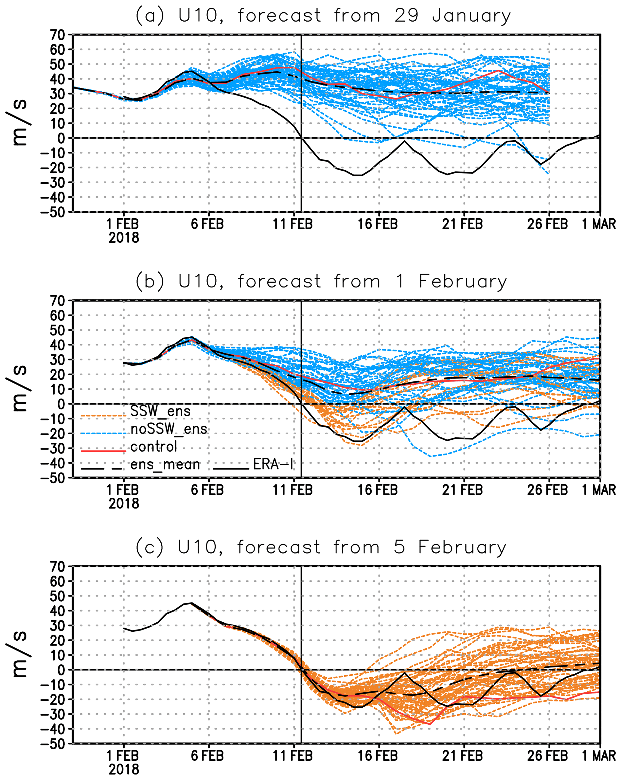
Figure 1 Zonal-mean zonal wind at 10 hPa and 60^∘ N (m s⁻¹). (a) Ensemble forecast initialized on 29 January; (b) ensemble forecast initialized on 1 February (orange lines denote ensemble members that predict wind reversal with max 1 d delay, red line – control forecast, black dashed line – ensemble mean) and the ERA-I reanalysis (black solid line); (c) forecast initialized on 5 February. Vertical line denotes the SSW2018 central date.

For the forecast verification, we use the ECMWF ERA-Interim reanalysis (ERA-I; Dee et al., 2011). The present analysis includes the period from 1979 to 2018. And 12-hourly data are used on a $\mathrm{1}{}^{\circ }\times \mathrm{1}{}^{\circ }$ horizontal grid covering the Northern Hemisphere (NH).

Stratospheric wind, eddy heat flux and wave-activity flux are analysed as full fields, while geopotential height is analysed as an anomaly except for Fig. 3. ERA-I anomalies are calculated with respect to the period 1997–2017, and the fields are detrended. The forecast anomalies are defined as the subtraction of the model's own climatology from the forecast fields. The model's own climatology is computed using hindcasts over the prior 20 years: 1997–2017.

We use the ensemble spread to assess the uncertainty in the forecast as small spread indicates high theoretical forecast accuracy, while large spread indicates low theoretical forecast accuracy. We show the ensemble spread in geopotential height, which is a measure of the difference between the members and is represented by the standard deviation with respect to the ensemble mean:

$$\begin{array}{}\text{(1)}& \mathrm{Spread}={\displaystyle \frac{\sqrt{\frac{\mathrm{1}}{N}\sum _{i=\mathrm{1}}^N\left(g_i-\stackrel{\mathrm{‾}}{g}\right)}}{\stackrel{\mathrm{‾}}{g}}},\end{array}$$

where g_i is geopotential height of an ensemble member, $\stackrel{\mathrm{‾}}{g}$ is ensemble mean and N is the number of ensemble members (N=51).

The wave-activity flux (WAF) indicates a propagating packet of planetary waves in three-dimensional space and is used to identify localized regions of wave-activity sources and sinks. Here we use the WAF F_s defined for quasi-stationary waves on a zonally varying basic flow following Takaya and Nakamura (2001):

$$\begin{array}{}\text{(2)}& \begin{array}{rl}& F_{\mathrm{s}}=\left(\begin{array}{c}{F}_x\\ F_y\\ F_z\end{array}\right)={\displaystyle \frac{p\cos \mathit{\phi }}{\mathrm{2}\left|u\right|}}\\ & \left(\begin{array}{l}\frac{u}{a^{\mathrm{2}}{\cos }^{\mathrm{2}}\mathit{\phi }}\left[{\left(\frac{\mathit{\delta }{\mathit{\psi }}^{\prime }}{\mathit{\delta }\mathit{\lambda }}\right)}^{\mathrm{2}}-{\mathit{\psi }}^{\prime }\frac{{\mathit{\delta }}^{\mathrm{2}}{\mathit{\psi }}^{\prime }}{\mathit{\delta }{\mathit{\lambda }}^{\mathrm{2}}}\right]+\frac{v}{a^{\mathrm{2}}\cos \mathit{\phi }}\left[\frac{\mathit{\delta }{\mathit{\psi }}^{\prime }}{\mathit{\delta }\mathit{\lambda }}\frac{\mathit{\delta }{\mathit{\psi }}^{\prime }}{\mathit{\delta }\mathit{\phi }}-{\mathit{\psi }}^{\prime }\frac{{\mathit{\delta }}^{\mathrm{2}}{\mathit{\psi }}^{\prime }}{\mathit{\delta }\mathit{\lambda }\mathit{\delta }\mathit{\phi }}\right]\\ \frac{u}{a^{\mathrm{2}}\cos \mathit{\phi }}\left[\frac{\mathit{\delta }{\mathit{\psi }}^{\prime }}{\mathit{\delta }\mathit{\lambda }}\frac{\mathit{\delta }{\mathit{\psi }}^{\prime }}{\mathit{\delta }\mathit{\phi }}-{\mathit{\psi }}^{\prime }\frac{{\mathit{\delta }}^{\mathrm{2}}{\mathit{\psi }}^{\prime }}{\mathit{\delta }\mathit{\lambda }\mathit{\delta }\mathit{\phi }}\right]+\frac{v}{a^{\mathrm{2}}}\left[{\left(\frac{\mathit{\delta }{\mathit{\psi }}^{\prime }}{\mathit{\delta }\mathit{\phi }}\right)}^{\mathrm{2}}-{\mathit{\psi }}^{\prime }\frac{{\mathit{\delta }}^{\mathrm{2}}{\mathit{\psi }}^{\prime }}{\mathit{\delta }{\mathit{\phi }}^{\mathrm{2}}}\right]\\ \frac{f_{\mathrm{0}}^{\mathrm{2}}}{N^{\mathrm{2}}}\left\{\frac{u}{a\cos \mathit{\phi }}\left[\frac{\mathit{\delta }{\mathit{\psi }}^{\prime }}{\mathit{\delta }\mathit{\lambda }}\frac{\mathit{\delta }{\mathit{\psi }}^{\prime }}{\mathit{\delta }z}-{\mathit{\psi }}^{\prime }\frac{{\mathit{\delta }}^{\mathrm{2}}{\mathit{\psi }}^{\prime }}{\mathit{\delta }\mathit{\lambda }\mathit{\delta }z}\right]+\frac{v}{a}\left[\frac{\mathit{\delta }{\mathit{\psi }}^{\prime }}{\mathit{\delta }\mathit{\phi }}\frac{\mathit{\delta }{\mathit{\psi }}^{\prime }}{\mathit{\delta }z}-{\mathit{\psi }}^{\prime }\frac{{\mathit{\delta }}^{\mathrm{2}}{\mathit{\psi }}^{\prime }}{\mathit{\delta }\mathit{\phi }\mathit{\delta }z}\right]\right\}\end{array}\right),\end{array}\end{array}$$

where F_x, F_y and F_z denote the zonal, meridional and vertical components of the wave-activity flux, respectively; p is pressure; φ and λ are latitude and longitude, respectively; u and v are zonal and meridional winds, respectively; $z=-H\ln \frac{p}{\mathrm{1000}\mathrm{hPa}}$ with constant scale height H; a is the Earth's radius; N is buoyancy frequency; and ψ is geostrophic streamfunction defined as $\mathit{\psi }=\mathrm{\Phi }/f$, where Φ is geopotential and f=2Ωsin φ is the Coriolis parameter (Ω is the Earth's rotation rate). The prime denotes perturbations from the zonal-mean values.

The Madden–Julian oscillation (MJO) phase is determined using the seasonally independent Real-time Multivariate MJO index (RMM) downloaded from the Australian Bureau of Meteorology (http://www.bom.gov.au/climate/mjo/, last access: 23 October 2020) for verification and from the Subseasonal-to-Seasonal Prediction Project (http://s2sprediction.net/, last access: 23 October 2020) for the forecasts. It is based on time series of the two leading principal components derived from empirical orthogonal functions (EOFs) of the combined fields of near-equatorially averaged 850 hPa zonal wind, 200 hPa zonal wind, and satellite-observed outgoing longwave radiation (OLR) data (Wheeler and Hendon, 2004). The RMM index is divided into eight phases that broadly correspond to the regions of enhanced convection.

3 Results

3.1 Stratospheric forecasts

We start by analysing the predictability of SSW2018 in the ECMWF ensemble forecast. Figure 1 shows the temporal evolution of the observed and forecasted zonal-mean zonal wind at 10 hPa and 60^∘ N (U10) for individual ensemble members during February 2018. In the forecast initialized on 29 January no members showed reversal to easterlies within 1 d from the observed onset date, although four members predicted an SSW to occur in the second half of February (Fig. 1a). In the forecast initialized on 1 February (Fig. 1b), there is a weak SSW signal: 14 ensemble members (∼27 %, orange dashed lines) predicted wind reversal within 1 d from the observed onset date. The forecasted SSW probability, defined as a fraction of ensemble members predicting an SSW at each day (Karpechko, 2018; Taguchi, 2016; Tripathi et al., 2016), was 0.06 on the observed onset date of 12 February and increased to 0.31 by 14 February when the minimum values of U10 were achieved by most ensemble members. The spread of predicted wind speed among the members increases markedly after 9 February when the observed polar night jet underwent the strongest deceleration. The fluctuations of the easterlies observed in the reanalysis after the reversal are not captured by any ensemble members. Karpechko et al. (2018) showed that most ensemble members underestimated the eddy heat flux at 100 hPa, which is used to characterize the upward planetary wave propagation from the troposphere to the stratosphere since it is proportional to the vertical group velocity of a planetary wave and to the vertical component of the Eliassen–Palm flux (Newman et al., 2001). With the reduction of the lead time, the prediction skill increases rapidly, and all ensemble members of the forecast initialized on 5 February capture the onset of the SSW (Fig. 1c). In this study we focus on the first ensemble forecast predicting the SSW (forecast from 1 February), and the contrast behaviour of the members that predicted and did not predict the event.

The evolution of zonal-mean zonal winds at 10 hPa for February 2018 is shown in Fig. 2. Early in the month, the axis of the polar night jet is located at around 70^∘ N and shifting gradually poleward (Fig. 2a). On 11 February, the jet quickly decelerates around 80^∘ N and the zonal wind reversal occurs in high latitudes and extends from the North Pole to about 50^∘ N. Easterly wind peaks of −30 m s⁻¹ are found on 12–16 February and around 21 February after diminishing to zero on 17 February at 60^∘ N. The northward shift of the polar night jet occurs prior to the zonal wind reversal – a feature highlighted in some previous SSW studies and pointed out as a precondition for the effective wave forcing, because in this case the relatively small mass and moment of inertia of the vortex allow upward-propagating waves to distort it (Limpasuvan et al., 2004; McIntyre, 1982; Harada et al., 2010; Nishii et al., 2009). The position of the vortex close to the pole and little vertical tilt are typical for the split SSWs as was pointed out by Albers and Birner (2014). Overall, easterly winds dominate the polar stratosphere north of 50^∘ N from mid-February to March.

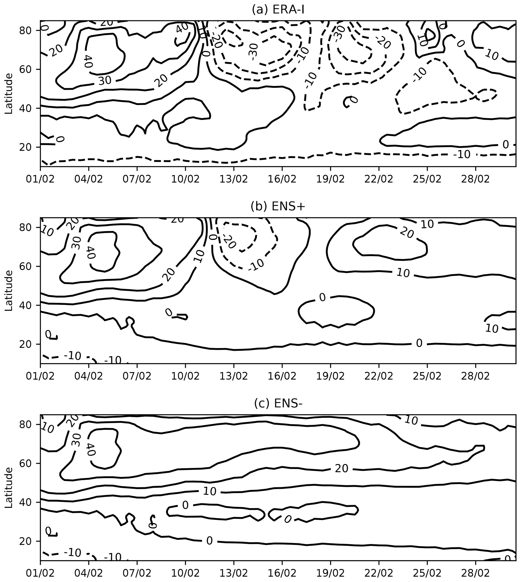
Figure 2 Latitude–time cross sections of zonal-mean zonal winds (m s⁻¹) at 10 hPa during February 2018. (a) ERA-I; (b) composite of ENS+ members; (c) composite of ENS− members. Contour intervals are 10 m s⁻¹.

The composite of the ENS+ members (Fig. 2b) captures well the northward shift of the polar jet axis in the beginning of February and the wind reversal on 12 February. The composite mean underestimates the magnitude and duration of easterlies, recovering to westerly flow after 18 February. This could possibly reduce the forecasted impacts of SSW2018 on the surface. Two ensemble members, however, maintained easterlies until the end of February, matching the magnitude of the observed easterlies, although neither of them captured the timing of the observed zonal-mean zonal wind oscillation during the negative phase (Fig. 1b). The ENS− composite (Fig. 2c) maintains westerlies throughout February.

Figure 3 shows that in the beginning of February the centre of the polar vortex is already displaced from the pole towards Greenland and the Norwegian Sea, and a high over Alaska begins to develop. During 4–6 February the two troughs over northern America and central Siberia and the anticyclone over Alaska start to form (not shown). By 7–9 February another high over the North Atlantic begins to develop (wavenumber 2 planetary wave pattern, Fig. 3a). During 10–12 February the two highs merge over the pole leading to a vortex split. The low over Canada intensifies while the other part of the split vortex weakens over Siberia, leading to the circulation reversal at 60^∘ N (Fig. 3d). To reveal forecast errors, we compare the ENS+ and ENS− members composites to the reanalysis (Fig. 3b, c, e and f). Analysis shows that during the first ∼7 d after the initialization the forecast errors in the stratosphere are modest, consistent with the analysis of Karpechko (2018), but they start to grow after 7 February mainly near the position of one of the daughter vortices over northern America in both ENS+ and ENS− clusters (Fig. 3b and c). By 10–12 February, the ENS− cluster notably underestimates the magnitude of the merged high that had replaced the polar vortex over the pole, and it shows bigger errors in the position of the cyclone over Canada (Fig. 3f) compared to the ENS+ cluster (Fig. 3e). However, the overall structure of the errors appears remarkably similar in the two groups, which might suggest the presence of a systematic model bias.

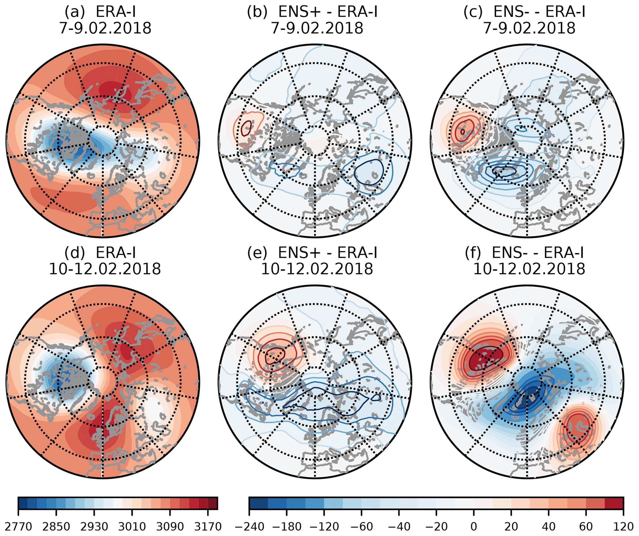
Figure 3 Geopotential height at 10 hPa (dam) for two successive 3 d means starting from 7 February (a, d). Difference in geopotential height at 10 hPa (dam) between ERA-I and ENS+ members (b, e) or ENS− members (c, f).

Long planetary waves are known to interact with the mean flow before SSWs (e.g. Limpasuvan et al., 2004). Time evolution of the planetary wave amplitudes in the beginning of February 2018 is shown in Fig. 4. The highest wave activity in the NH stratosphere is concentrated within the latitudinal range of 40–75^∘ N (e.g. Peters et al., 2010); therefore, this belt of latitudes was chosen for averaging. Planetary wave with wavenumber 1 (PW1) dominates in the beginning of February in the middle stratosphere, but its amplitude decreases rapidly and reaches its minimum on 10 February. On the other hand, the amplitude of PW2 starts to grow rapidly on 4 February, reaching values of 90 dam on 10 February just before the SSW2018 onset (Fig. 4a). Such inverse correlation of these two planetary waves is often observed before major split-type SSWs as the propagation characteristics of the waves differ, depending on the zonal wavenumber and wave period (Charney and Drazin, 1961). Moreover, the amplitude vacillation between PW1 and PW2 may be caused by wave–wave interactions (Smith, 1983). A strong PW2 increase often results in a vortex splitting (McIntyre, 1982), as it happened in February 2018. Figure 4b and c depict the time evolution on the first three waves for each of the 10 chosen ENS+ and ENS− members. First, the evolution across individual ensemble members in both categories is remarkably similar, though the spread in the ENS− cluster is bigger. The overall evolution pattern in the ENS+ cluster resembles well the ERA-I verification (Fig. 4b). The ENS− members fail to capture the amplitude growth of the PW1 after 10 February, and in addition to that, they underestimate the PW2 amplitude (Fig. 4c). PW3 remains weak in both observation and forecast ensembles.

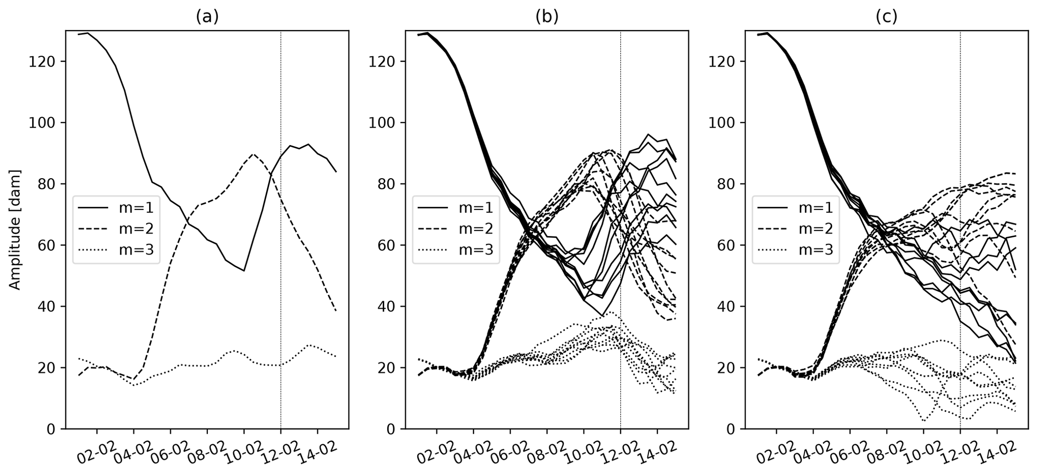
Figure 4 Time series of amplitudes of planetary waves with wavenumbers m=1, 2 and 3 in geopotential height (dam) at 10 hPa averaged over the latitudinal belt 40–75^∘ N (a) ERA-I reanalysis, (b) ENS+ members, (c) ENS− members. Vertical line denotes the SSW2018 central date.

On 7 February the polar vortex had already been weakened and distorted (Fig. 3a), and the polar night jet started to decelerate. Horizontal distribution of the ensemble spread in the lower stratosphere, represented by the standard deviation of the ensemble members, is shown in Fig. 5. The largest ensemble spread is mainly confined to the subpolar North Atlantic (Fig. 5a), where the forecast errors on that date are the largest (Fig. 3c). Throughout the period of vortex deceleration, the area of the large forecast spread at 50 hPa height gradually expands horizontally and, by 12 February, covers most of the polar stratosphere north of 70^∘ N (Fig. 5b and c).

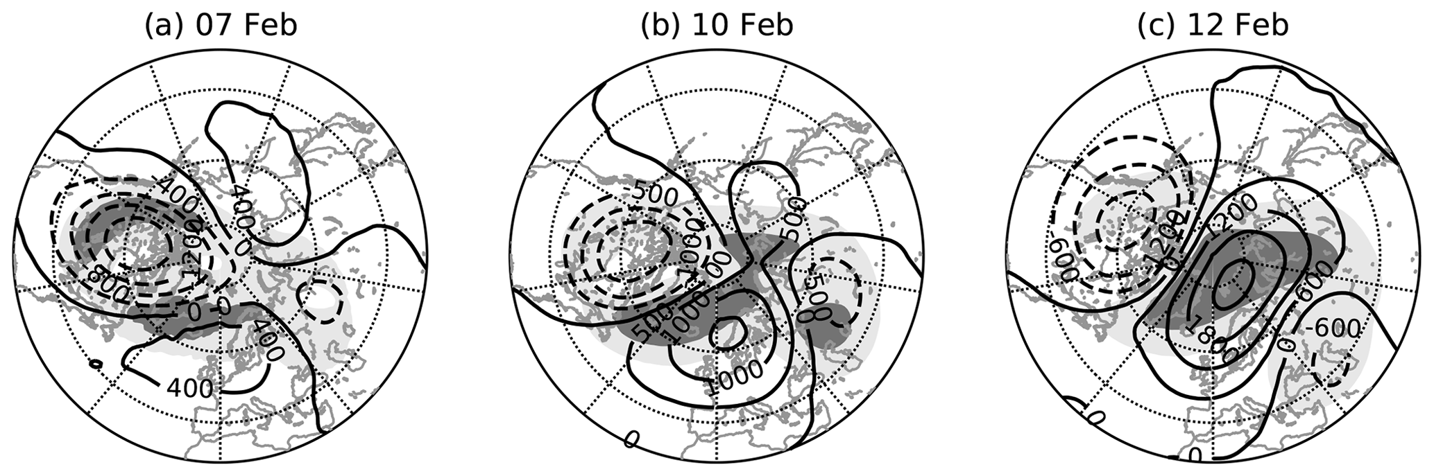
Figure 5 ERA-I 10 hPa geopotential height anomalies (contours, m) with respect to the 1980–2010 climatology and ensemble spread of geopotential height predicted for (a) 7, (b) 10 and (c) 12 February 2018 (shaded lightly and heavily for 0.3–0.6 values and values greater than 0.6, respectively). The spread has been normalized by the minimum and maximum values within the domain north of 20^∘ N.

To better understand sources of ensemble spread in the stratosphere, we look at the zonal cross sections (Fig. 6). As seen in Fig. 6a, there are three areas of large ensemble-forecast spread on 7 February, when the polar vortex started to decelerate and be distorted: over the Ural Mountains, Alaska and North Atlantic regions. The areas with the large spread extend from the troposphere into the lower stratosphere. Blocking anticyclones in these regions were pointed out to be associated with SSW tropospheric forcing (Martius et al., 2009; Woollings et al., 2010; Rao et al., 2018; Karpechko et al., 2018), as they may act as the source of the Rossby wave packets that propagate into the stratosphere and lead to a SSW onset. The upward group velocity propagation of the waves is indicated by the westward tilt of the geopotential anomaly lines with height (Fig. 6). The spread can be explained by the inconsistencies in the location, amplitudes and group velocities predicted by different ensemble members (Nishii and Nakamura, 2010). In fact, most of the ensemble members started to underestimate the heat flux entering the stratosphere (Fig. 1 in Karpechko et al., 2018) after 7 February.

Figure 6 Zonal cross sections for 50^∘ N of the ensemble spread of geopotential height predicted for (a) 7, (b) 10 and (c) 12 February 2018. Superimposed contours represent observed geopotential anomalies (m) with respect to the 1980–2010 climatology. Solid lines represent anticyclonic (positive) anomalies and dashed lines cyclonic (negative) anomalies. Anomaly is normalized by pressure.

To further analyse the contribution of these three regions to the SSW2018 forcing, we examine the time series of the vertical component of wave-activity flux averaged zonally and over the three continuous longitudinal ranges. The main wave event is identifiable in the lower and middle stratosphere prior to the circulation reversal (Fig. 7a), preceded by the upward flux maxima in the lower and mid-troposphere on 4 February with the time lag of ∼7 d needed for the planetary wave to propagate vertically from the troposphere to the stratosphere. The division into three longitudinal ranges allows us to investigate the wave-activity flux propagation between the troposphere and the lower and middle stratosphere over the limited longitudinal ranges (Harada et al., 2010; Coy and Pawson, 2015). The North Atlantic sector (Fig. 7j) shows the biggest maxima of vertical wave-activity flux in the troposphere in the beginning of February and also in the lower and middle stratosphere just before the SSW onset compared to the other two-thirds of the globe. Strong upward propagation can also be seen in the stratosphere in the Europe/Siberia sector, which likely contributed to initial weakening of the vortex (Fig. 7d). The North Pacific sector (Fig. 7g) shows an increased upward flux before the event, which is restricted to the lower stratosphere. Additional analysis showed that wavenumber 2 was the largest contributor to the upward wave activity during the week preceding SSW, while wavenumber 1 was the largest contributor until 3–5 February (not shown), which is in agreement with wave amplitude evolution shown in Fig. 4. Note that enhanced tropospheric forcing, in addition to directly affecting the mean stratospheric circulation, may also alter the geometry of the vortex and precondition it to splitting by triggering the internal resonance (Albers and Birner, 2014).

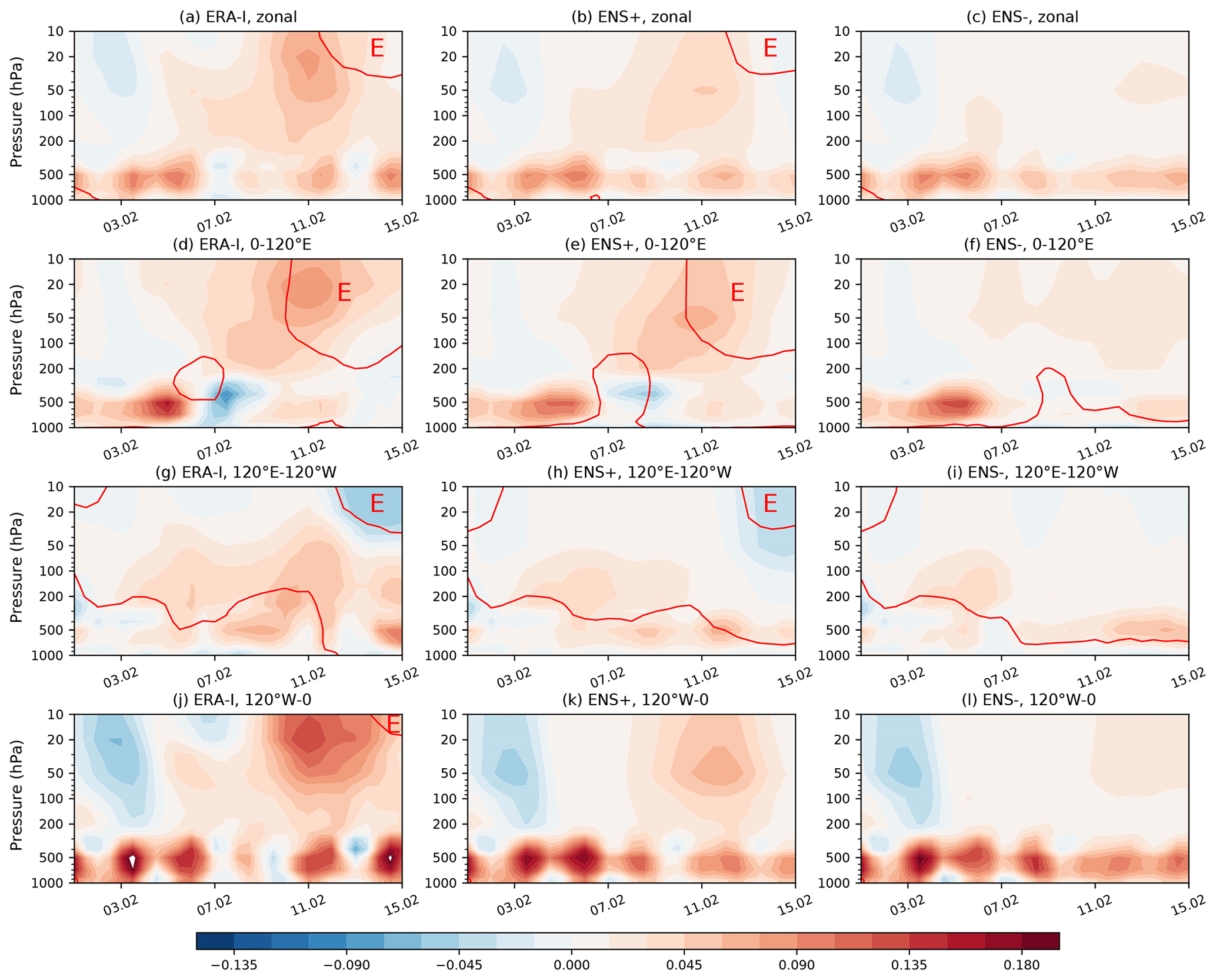
Figure 7 Time–altitude plot of the vertical component of WAF (m² s⁻², shaded, averaged over 45–90^∘ N, vertically scaled by $\sqrt{\text{(1000\hspace{0.17em}hPa)}/p}$) and zero zonal wind contour (red) averaged over 55–65^∘ N. (a–c) Zonally averaged; (d–f) averaged over 0–120^∘ E; (g–i) averaged over 120^∘ E–120^∘ W; (j, i) averaged over 120–0^∘ W. The red letter “E” denotes regions of easterly winds. (a, d, g, i) ERA-I; (b, e, h, k) ENS+ composite; (c, f, i, l) ENS− composite.

Comparison of the similar diagnostics of vertical WAF performed for the ENS+ and ENS− composites (Fig. 7, second and third columns, respectively) shows that the ENS+ cluster captures the wave propagation patterns zonally averaged (Fig. 7b) and in all three longitudinal ranges (Fig. 7e, h and k), although it somewhat underestimates the magnitudes of fluxes. The ENS− forecast composite does not predict a significant vertical wave propagation from the troposphere into the stratosphere in either of the longitudinal ranges.

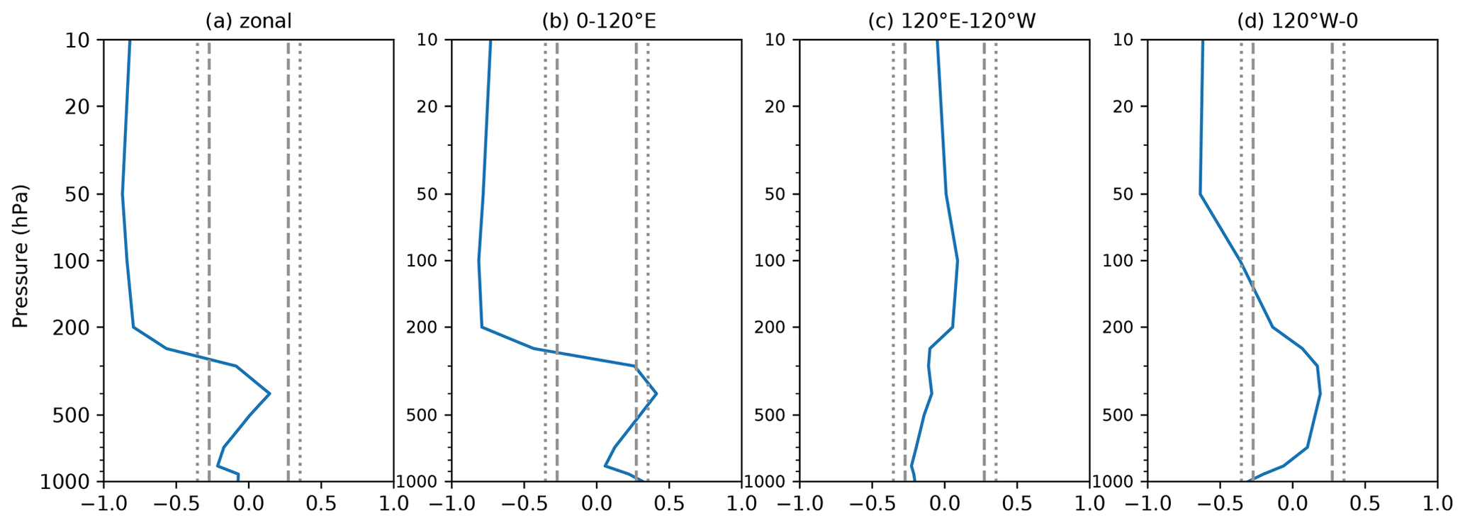
Figure 8 Vertical distribution of the correlation coefficient between the vertical component of the WAF forecasts averaged during 4–11 February and U10 forecasts valid on 12 February across individual forecast ensemble members. (a) Zonally averaged; (b) averaged over 0–120^∘ E; (c) averaged over 120^∘ E–120^∘ W; (d) averaged over 120–0^∘ W. Dashed vertical lines denote the 0.05 significance level; dotted vertical lines denote the 0.01 significance level.

While the ENS− forecasts failed to reproduce the increases in wave-activity flux in all three regions, it is not clear where the errors were crucial for the failed SSW forecast. The correlation analysis of the zonal-mean WAF at each level averaged over 4–11 February with forecast U10 on 12 February across individual ensemble members shows the negative correlation, starting from the upper troposphere, at the 0.05 significance level (Fig. 8a). The correlation coefficient increases with height, reaching $r=-\mathrm{0.9}$ at 50 hPa. When split into the three regions, the wave-activity contributions from the Siberia and North Atlantic sectors are significant in the lower and middle stratosphere, with strongest negative correlations found in the Europe/Siberian sector (Fig. 8b). This suggests that upward wave-activity propagation in these regions was critical for the SSW2018 forcing. On the other hand, the correlation analysis shows that there is no significant relation between WAF in the North Pacific sector (Fig. 8c) and U10.

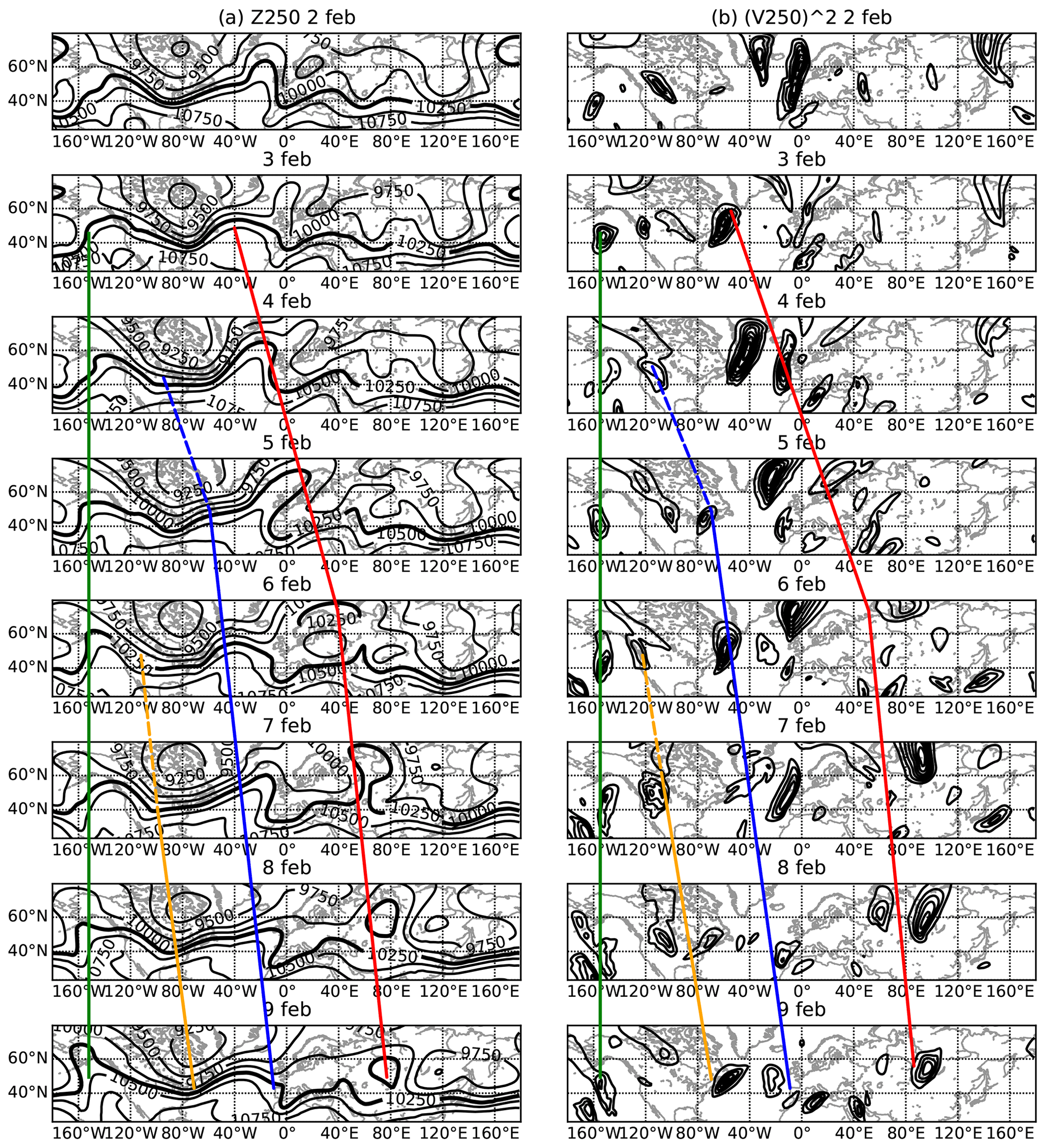
Figure 9 Time sequence of (a) ERA-I 250 hPa geopotential height observed from 2 (top) to 9 (bottom) February 2018 over a domain (20–70^∘ N). The thick contour corresponds to 10 250 m. (b) ERA-I 250 hPa meridional velocity squared; contour intervals are 800 m² s⁻². The coloured lines track the movement of the ridges and troughs (a) and corresponding maxima of meridional velocity squared (b), and they suggest the propagation of wave packets.

3.2 Tropospheric waves

We next look at the tropospheric precursors of SSW2018. The three areas with the largest forecast spread (Fig. 6) are associated with blocking ridges seen in the 250 hPa geopotential height (Fig. 9a). Several wave packets manifested as meandering westerlies can be distinguished in the consecutive geopotential height fields over the period of 3–9 February (coloured lines). The most pronounced one is associated with the anticyclonic wave-breaking episode over the North Atlantic (red line) also demonstrated by Lee et al. (2019). Here, a well-developed ridge can be seen on 3 February. During 4–6 February this ridge breaks anticyclonically and forms a cut-off anticyclone over Scandinavia on 6 February, which continued propagating downstream until blocked over the Ural region around 7 February after which time it remained quasi-stationary until 9 February (red line). The second ridge (blue line) can be distinguished propagating across the North Atlantic during 5–8 February until it decayed over Spain on 9 February. The developing of this wave might be traced back in squared meridional wind to western North America on 4 February (dashed blue line in Fig. 9b). Finally, a trough can be seen propagating across North America during 7–9 February (yellow line). Its development can also be traced in squared meridional wind back to western North America on 6 February. At the same time a stationary upper troposphere ridge is seen over Alaska over the whole period (green line).

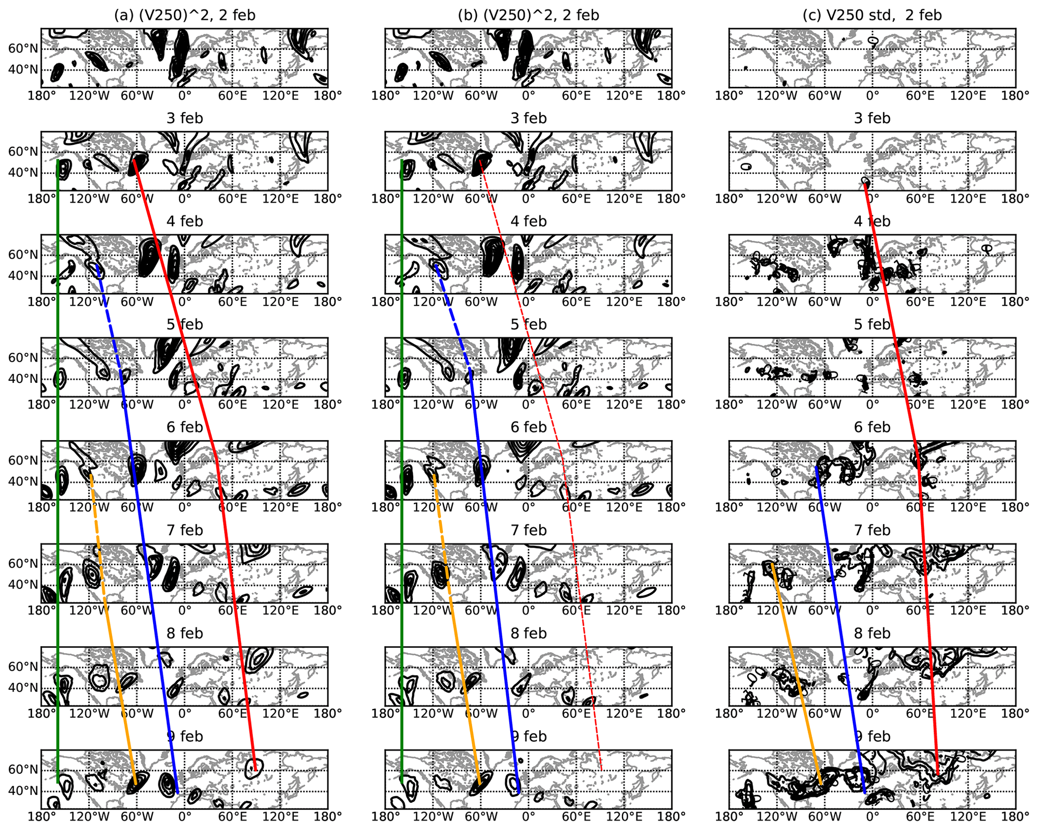
Figure 10 Same as Fig. 9b but for ENS+ (a) and ENS− (b) members; contour intervals are 800 m² s⁻²; (c) standard deviation of the predicted 250 hPa meridional wind velocity among ensemble members. The standard deviation is normalized by the maximum and minimum within the domain. Contour intervals are 0.1 starting from 0.5. The coloured lines are mostly similar to those in Figure 9 and suggest the propagation of wave packets. The red line in (b) is dashed to emphasize the lack of this wave train in ENS−. The green line in (c) is missing because there is little forecast spread in the eastern Pacific.

The propagation of the synoptic features can be also diagnosed using the squared meridional wind fields (Nishii and Nakamura, 2010). Figure 9b shows that, between 3 and 7 February, the maximum of the squared 250 hPa meridional wind propagated across the North Atlantic and northern Eurasia with an average group speed of ∼27^∘ in longitude per day before being blocked over the Urals with little downstream propagation thereafter. Such propagation speed is consistent with group velocity of baroclinic waves (Chang, 1993; Nishii and Nakamura, 2010), suggesting that formation of the blocking anticyclone was the result of a downstream development. Figure 9b also shows that the stationary Alaskan ridge served as a source of two more individual wave packets that propagated towards the Atlantic starting on 3 and 6 February.

The ENS+ composite of the squared meridional wind at 250 hPa (Fig. 10a) is in agreement with the reanalysis (Fig. 9b), capturing all three wave packets discussed above, whereas in the ENS− cluster the wave train over the Ural region disappears starting from 6 February. Thus, the wave packet associated with the Ural blocking fades away in the ENS− members. Although the propagation of other wave packets is captured by the ENS− cluster, there are differences with respect to the ENS+ cluster in the location and magnitude of the packets. In particular the magnitude of the Atlantic ridge on 6–9 February is strongly underestimated. The differences between the ENS+ and ENS− clusters can also be investigated by looking at the forecast spread in the meridional wind at 250 hPa that represent inconsistency among the ensemble members (Fig. 10c). Downstream propagation of the forecast spread is well distinguishable in Fig. 10c, and it is strongly associated with the propagation of the aforementioned wave packets. Interestingly, there is large spread also in the eastern Pacific associated with the quasi-stationary Alaskan ridge.

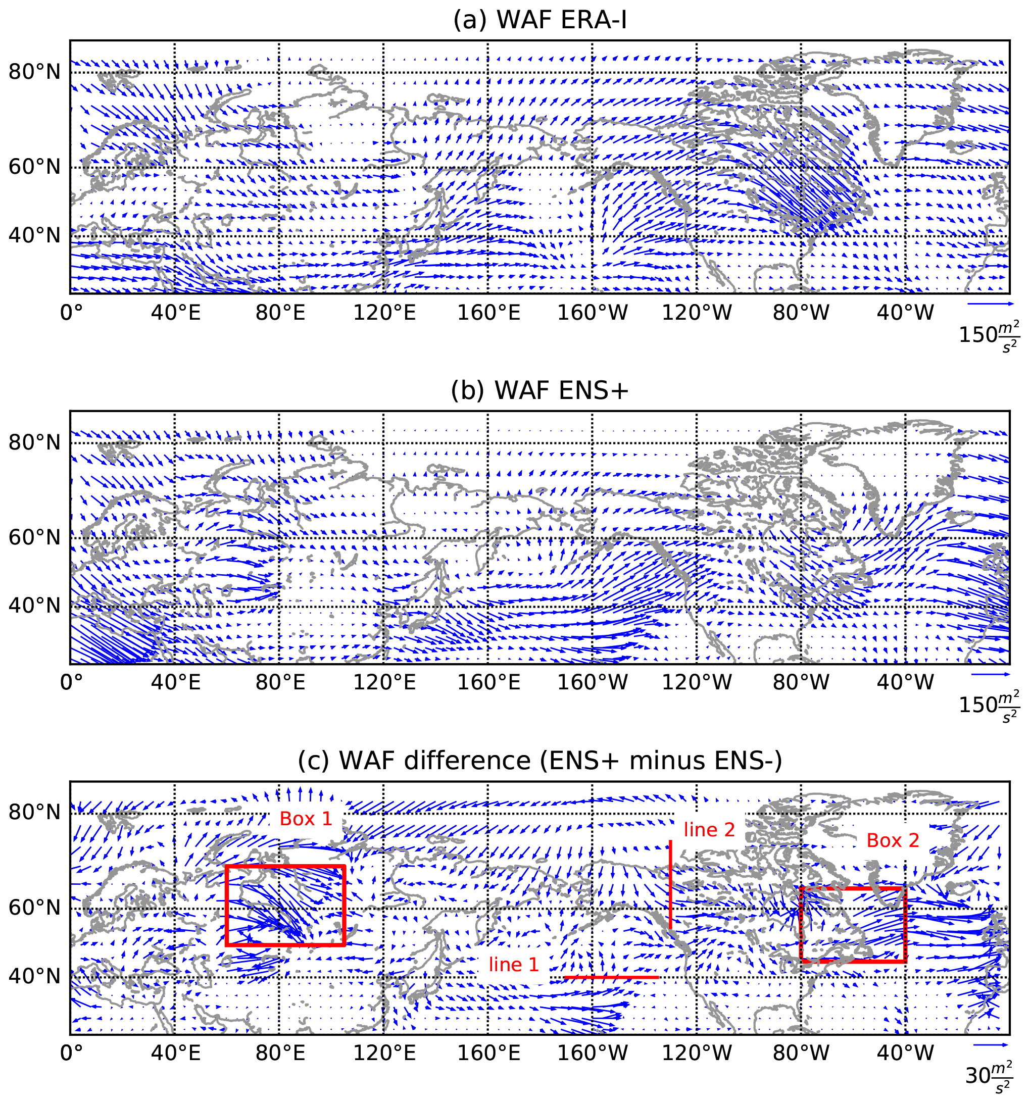
Figure 11 The 500 hPa horizontal WAF (m² s⁻²) averaged over 5–7 February. (a) ERA-Interim; (b) ENS+; (c) difference between ENS+ and ENS− groups of ensemble members.

To see the behaviour of the wave packets in more detail, we studied the horizontal propagation of WAF. The observed wave activity in the mid-troposphere and the difference between the ENS+ and ENS− clusters are shown in Fig. 11 for 5–7 February. We focus on this time period because this is when large differences between these two ensembles have emerged, and we use 3 d averaging following previous practices of using this diagnostic developed for quasi-stationary waves (e.g. Harada et al., 2010; Peters et al., 2010). The 500 hPa pressure level is chosen to highlight the mid-tropospheric processes. The same diagnostics in the upper troposphere (300 hPa) yield similar results (not shown). Figure 11a shows eastward propagation of wave activity along the jet stream in the reanalysis, with large values seen in all three regions of anomalous highs identified in the previous sections. The wave-activity propagation in the ENS+ members group is reasonably similar to the reanalysis (Fig. 11b). However, the eastward WAF is stronger in the ENS+ members compared to ENS− through most of the NH extratropics with the greatest differences following the meandering extratropical jet stream (Fig. 11c). Remarkable difference in the horizontal propagation of wave packets is seen over all three centres of forecast uncertainty discussed above – Alaska, North Atlantic and Urals, suggesting underestimation of eastward wave-activity propagation in the ENS− cluster. To inspect closely the difference in wave propagation between the ENS+ and ENS− clusters, we look at the magnitude of the horizontal wave flux within the areas representative of these regions marked in Fig. 11c as two boxes (over the Ural region – box 1 – and the North Atlantic – box 2). Over the North Pacific, since the anomalous flux changes its direction within the area, we choose to analyse the flux through the two surface lines (Fig. 12). The wave-activity propagation over the box 1 in the ENS+ cluster captures well the sharp amplification seen in the ERA-I verification between 5 and 9 February and somewhat overestimates its magnitude. This amplification corresponds to the period of the development of the Ural blocking high (Fig. 12a). The ENS− cluster fails to capture this intensification of the wave activity. The wave-activity fluxes through the surfaces, defined by lines 1 and 2 (Fig. 12b and c), are comparable between the ENS+ and ENS− clusters and reproduce the fluctuations seen in ERA-I. Note that this result is not sensitive to the exact location of the lines. The analysis of the net flux in the North Atlantic region (box 2) shows the two individual peaks between 3 and 9 February, corresponding to the joint effect of the three individual wave packets revealed in Figs. 9 and 10, which are somewhat underestimated in both ensemble members groups (Fig. 12d). Thus, results in Fig. 12 suggest that the key difference between the ENS+ and ENS− forecasts in terms of horizontal wave-activity propagation is in the Ural region.

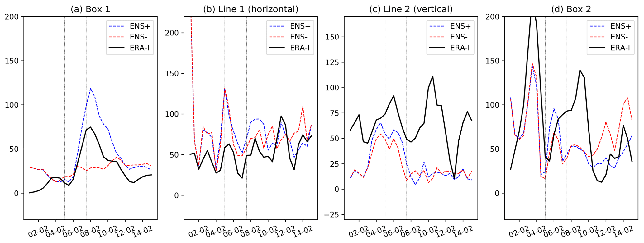
Figure 12 Time series of the horizontal WAF at 500 hPa (m² s⁻²) averaged over boxes 1 and 2 and through lines 1 and 2 shown in Fig. 11c. Panels (a) and (d) show mean length of the horizontal WAF vector, while panels (b) and (c) show mean meridional and zonal components, respectively. Grey vertical lines denote the averaging period taken for analysis in Fig. 11: 5 and 7 February.

To demonstrate that the differences in horizontal WAF in the mid-troposphere between the ENS+ and ENS− clusters are relevant for SSW forecasting, we perform the correlation analysis of zonal-mean zonal wind in the mid-stratosphere and the zonal component of WAF at 500 hPa across all ensemble members. The correlation field (Fig. 13) has two centres of negative correlations – over the North Atlantic and Ural regions with statistically significant correlation coefficients exceeding −0.5. These centres coincide with the locations of the biggest differences in WAF between the ENS+ and ENS− clusters (Fig. 11). The negative correlations indicate that the stronger flux in the regions is associated with weaker stratospheric winds and suggest that errors in the wave activity in the location of the Ural high and Atlantic storm track were crucial for forecasting SSW2018, consistent with the results by Karpechko et al. (2018) and Lee et al. (2019).

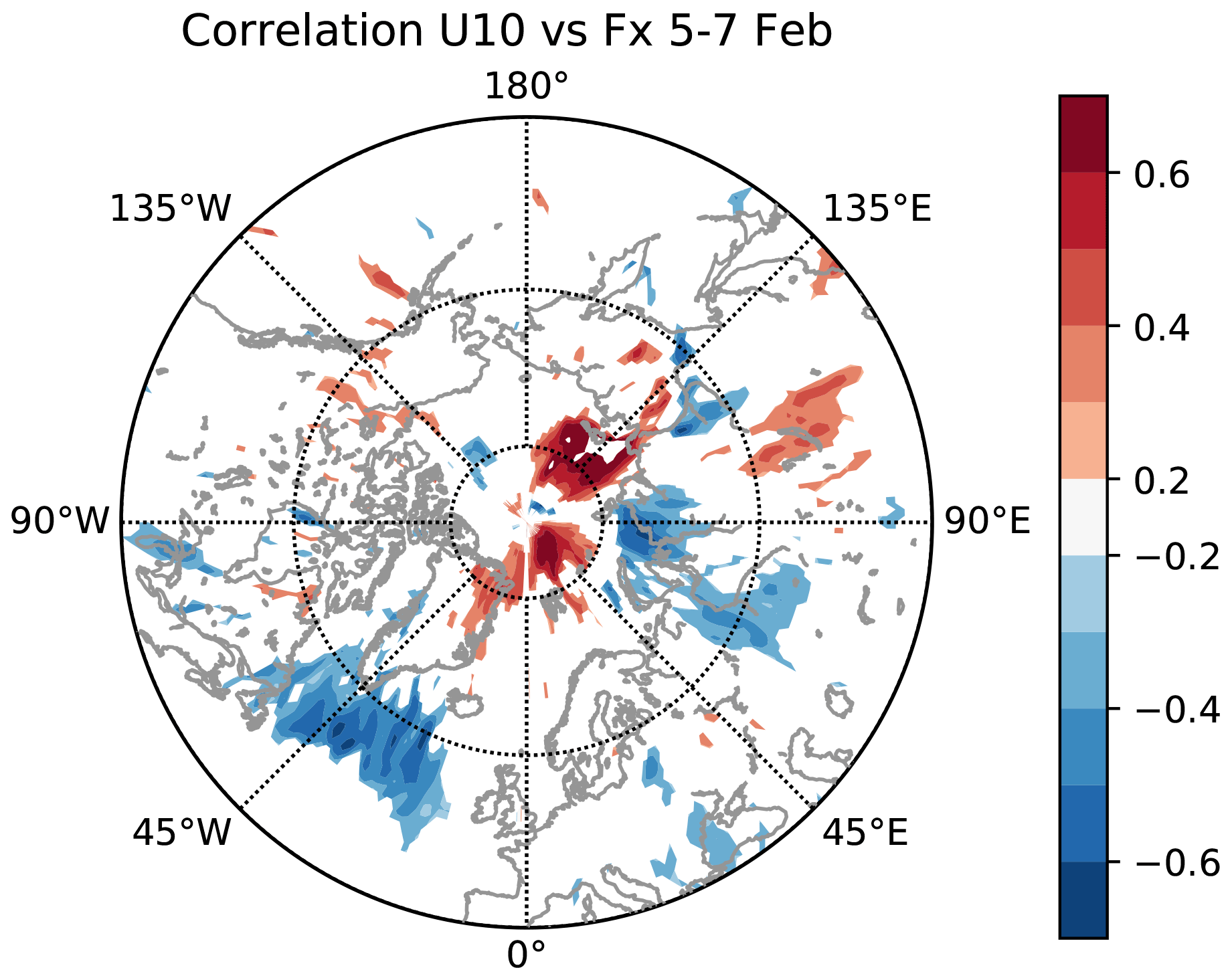
Figure 13 Correlation coefficient between zonal WAF at 500 hPa averaged 5–7 February and U10 reanalysis on 12 February across individual ensemble members. All shaded coefficients are significant at p=0.05.

3.3 Teleconnection with MJO

Before the SSW2018 central date, an active MJO in phases 6 and 7 with large amplitude prevailed in the tropical Indian Ocean and South China Sea (Barrett, 2019). It has been shown that MJO phase 6 and 7 events associated with OLR anomalies in the eastern Pacific can lead to weakening of the polar vortex through enhancement of upward-propagating wave fluxes towards Alaska and are often followed by SSWs (Schwartz and Garfinkel, 2017). In this section we assess the evidence that the MJO played a role in the onset of SSW2018. We chose for the analysis the ensemble forecast initialized on the 1 February, and as the amplification of the MJO phase 6 occurred prior to that date, it is expected that the wave-activity source associated with MJO has been included into forecast initial conditions, potentially leading to the more precise forecast of SSW2018. We find no evident link between the skill of MJO forecast and SSW2018: the ENS+ members do not predict MJO more correctly that the ENS− members (see Fig. A2). Based on that we focus on analysis of MJO teleconnections, testing the hypothesis that correct forecasting of MJO teleconnections was an important factor in simulating SSW2018.

To verify that, we first constructed the composite field of geopotential height anomalies picked only for days with MJO phase 6 with the lag of 5–9 d in both ECMWF historical forecasts and ERA-I. It is very difficult to clearly establish the causality between tropical oscillations and polar anomalies because of the complex interactions between the propagating waves and the mean flow. Therefore, one of the ways to approach causality is to use time lag. The lag of 5–9 d after MJO phase 6, which took place on 27–31 January, roughly corresponds to the period in early February when tropospheric waves forced SSW2018 based on the analysis in the previous sections. In particular, the ridge over the North Atlantic was developing during this period. This suggests that the MJO phase 6 fingerprint should be taken with the lag of 5–9 d.

We start by testing how well the model can reproduce MJO phase 6 teleconnection in the extratropics. In Fig. 14a contours represent the composite fields showing the climatological ERA-I fingerprints of the MJO phase 6. Contours in Fig. 14b and c show similar fingerprint but constructed with the model hindcasts over the 20-year period. These two fields both have prominent lows in the North Pacific and over Canada and highs over the Ural, western North America and the North Atlantic. Although the fingerprint fields show some dissimilarity in the positions and strength of the features, their overall structure is well captured by the model. This result is in line with Vitart (2014, 2017), who showed that the model produces realistic patterns of MJO teleconnections.

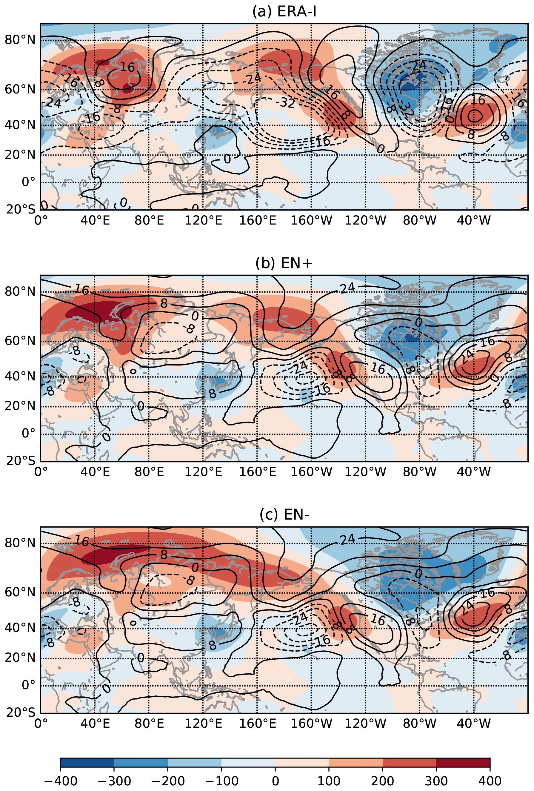
Figure 14 Geopotential height anomalies at 500 hPa in (a) ERA-I, (b) ENS+ members and (c) ENS− members. Contours show geopotential height composite (m) for MJO phase 6 averaged over lags of 5–9 d. Shading shows anomalies averaged over 5–7 February 2018. ERA-I composites are calculated using 1997–2017 data. Forecast model composites are calculated using hindcasts over the same period.

Figure 14a also shows the observed geopotential anomalies field averaged for 5–7 February (shading), i.e. 5–7 d after the end of the MJO phase 6. Although the key features in 2018 are somewhat displaced with respect to the climatological composite, the overall structure of the field prior to SSW2018 strongly resembles the climatological MJO response, capturing the anomalous highs over Siberia, high-latitude Pacific and North Atlantic, as well as the low over Canada. The spatial correlation between the two fields (climatological lagged composite for phase 6 and anomalies observed on 5–7 February 2018) in the extratropics (40–90^∘ N) is r=0.32 and significant at the 0.01 level. On the other hand, the low in the North Pacific region is not pronounced and the high over western America is displaced towards the north-west. Although the evidence is not conclusive, the similarity between the pattern observed in early February 2018 and the climatological MJO phase 6 signal support the idea that MJO teleconnections may have played a significant role in dynamical evolution of the extratropical atmosphere during early February 2018, and therefore could contribute to forcing of SSW2018, consistent with existing literature (Schwartz and Garfinkel, 2017).

The composite field made for 5–7 February 2018 using the ENS+ members captures the observed structure of geopotential height field well with PW2 pattern prevailing in the northern latitudes and also strongly resembling the MJO fingerprint composite (Fig. 14b). On the contrary, the response in the ENS− cluster shows a PW1 pattern with two highs in Alaska and the Ural region that merged together (Fig. 14c), which is consistent with the ENS− forecasts not capturing the amplification of PW2 in the stratosphere (Fig. 4c). In summary, our composite analysis provides supportive, although not decisive, evidence that teleconnections associated with MJO phase 6 played a role in triggering SSW2018 both in observations and in the forecasts.

4 Discussion and conclusions

Using the ECMWF ensemble forecast, we examined the predictability of the major SSW in the middle of February 2018. We focused on the identification of the involved dynamical processes and studied the role of the tropospheric forcing leading to the polar vortex split.

First, we have selected two groups of ensemble members based on the zonal-mean zonal wind at 10 hPa and 60^∘ N metric to discern the spatial and temporal distribution of forecast errors and its possible sources by comparing the ensemble composites to the reanalysis fields. SSW2018 was preceded by the amplification of PW2 and record-breaking eddy heat flux in the lower stratosphere. This amplification was reasonably well captured by forecast ensemble members predicting SSW2018 but not those that did not predict it (Fig. 4). The forecast error in geopotential height in the mid-stratosphere is small until 7 February and starts to grow mainly near the edge of the polar vortex following its displacement towards North America (Fig. 3), which is marked also by the largest ensemble spread (Fig. 5). The growth of the forecast spread was linked to the positions of tropospheric blocking ridges (Fig. 6), suggesting that their accurate prediction was important for forecasting the SSW2018 event. The amplification of the stratospheric PW2 was related to a PW2 pattern in the mid-troposphere and was apparently brought about by accumulative effects of localized propagation of wave packets. The period preceding SSW2018 was characterized by the enhanced wave activity in the troposphere. In the Pacific region wave-activity fluxes maintained a quasi-stationary ridge over Alaska (Fig. 7). Over the North Atlantic, eastward propagation of individual wave packets could be identified and tracked back to the Alaskan ridge, which served as their source. We show that the propagation of the forecast uncertainties is associated with the downstream propagation of these synoptic patterns in the troposphere, and the subsequent upward propagation of the wave packets to the stratosphere. Comparison of the ENS+ and ENS− forecast composites reveals that the ENS+ forecasts correctly captured the whole chain of the observed events: from downstream propagation of individual wave packets to the upward propagation of wave activity, amplification of stratospheric PW2 and breaking down of the stratospheric polar vortex. On the other hand, our analysis suggests that ENS− members underestimated both horizontal and vertical WAF propagation. In particular, it is found that the development of the upper troposphere blocking anticyclone over the Ural region around 6–7 February following the energy injection from wave breaking over the North Atlantic during 4–6 February was largely missing in the ENS− cluster. This wave-breaking event was also highlighted by Lee et al. (2019) as being important for amplifying a high-pressure system over the Urals and triggering SSW2018. We have also shown that the wave packet crucial for the formation of the Ural blocking is not captured by the ensemble members that failed to forecast SSW2018. According to our statistical analysis, forecasted stratospheric winds are mostly correlated with horizontal zonal wave-activity flux over the Ural region, with stronger WAF in that region being associated with weaker stratospheric winds (Fig. 13). Furthermore, correlation analysis also reveals that weaker stratospheric winds in the forecast were mostly associated with the vertical propagation of the wave-activity flux over the Siberian sector with a contribution from the North Atlantic sector (Fig. 8). While we also find enhanced vertical wave-activity propagation from the Alaskan sector, correlation analysis of the forecast members suggests that WAF over this region did not contribute to the SSW2018 forcing, which is somewhat inconsistent with results by Rao et al. (2018), who concluded that SSW2018 is caused by the Alaskan blocking.

SSW2018 was preceded by the highest ever observed MJO phase 6, which could create favourable conditions for strengthened Rossby wave teleconnections between the tropics and the extratropics. We have shown that the anticyclonic centres over the North Atlantic, Ural and Alaskan regions formed before SSW2018 correspond to the MJO phase 6 response pattern taken with the lag of 5–9 d (Fig. 14). These centres were captured well by the ENS+ members, while the ENS− cluster failed to reproduce the PW2 structure in the northern latitudes. The composite analysis provides evidence, albeit indecisive, that teleconnections associated with MJO phase 6 played a role in triggering SSW2018.

We conclude by pointing out the importance of the accurate prediction of the strength and position of synoptic-scale mid- and upper-tropospheric features and understanding of the origin of planetary wave anomalies for improving the prediction of SSW events. Although the predictability of the 1–2 weeks for SSW2018 falls within the usual range of predictability for the split events (Karpechko, 2018; Domeisen et al., 2020), the exceptional conditions before the event could have potentially enhanced the predictability. It is important to understand what part of the forecast error was associated with internal variability and what part was due to systematic bias, which is planned to be addressed in a follow-up study.

Appendix A

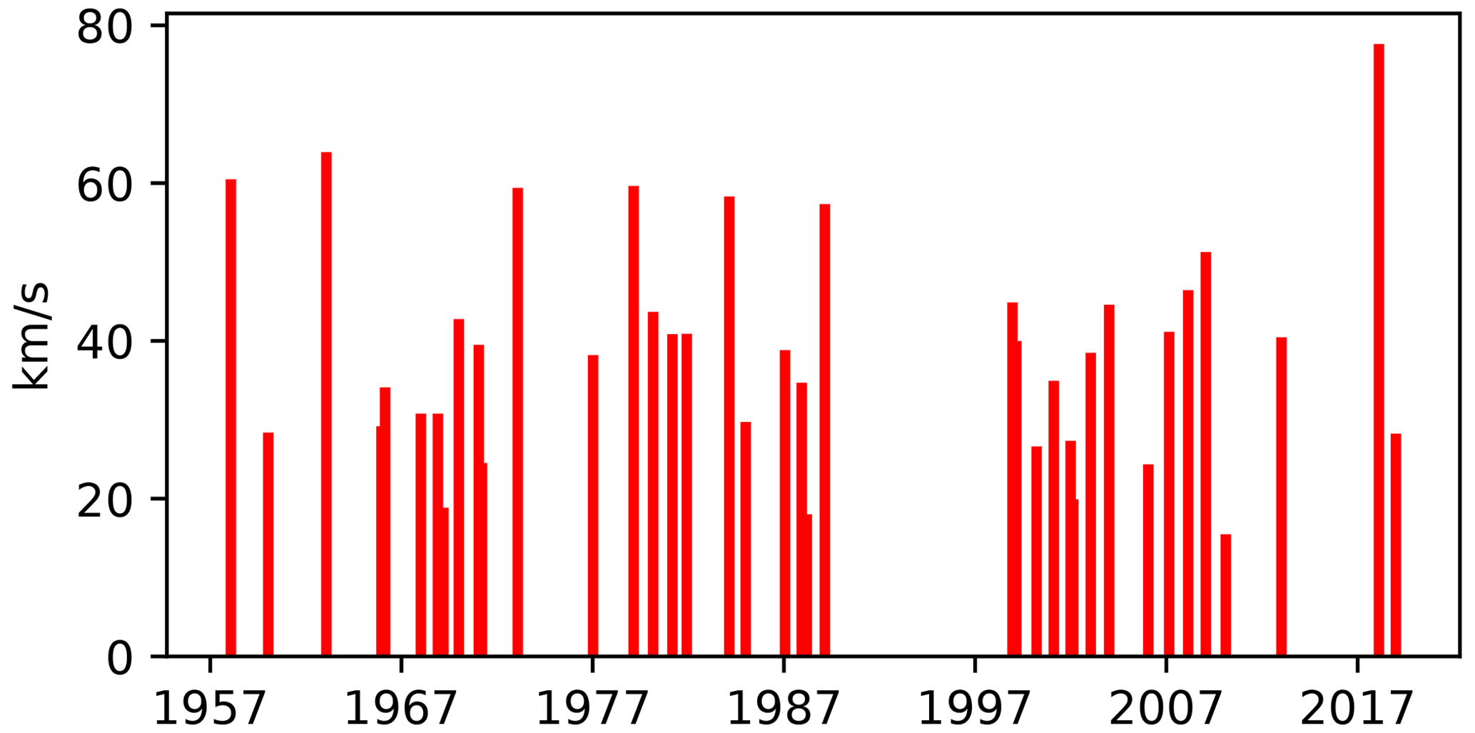
Figure A1 Eddy heat flux at 100 hPa (km s⁻¹) averaged across 50–75^∘ N observed over 5 d prior to a major SSW during 1958–2018. The dates of the SSWs are taken from Charlton and Polvani (2007) and Karpechko (2018). The heat flux in 1979–2018 was calculated using ERA-I reanalysis, while in 1958–1978 it was using the ERA-40 reanalysis (Uppala et al., 2005).

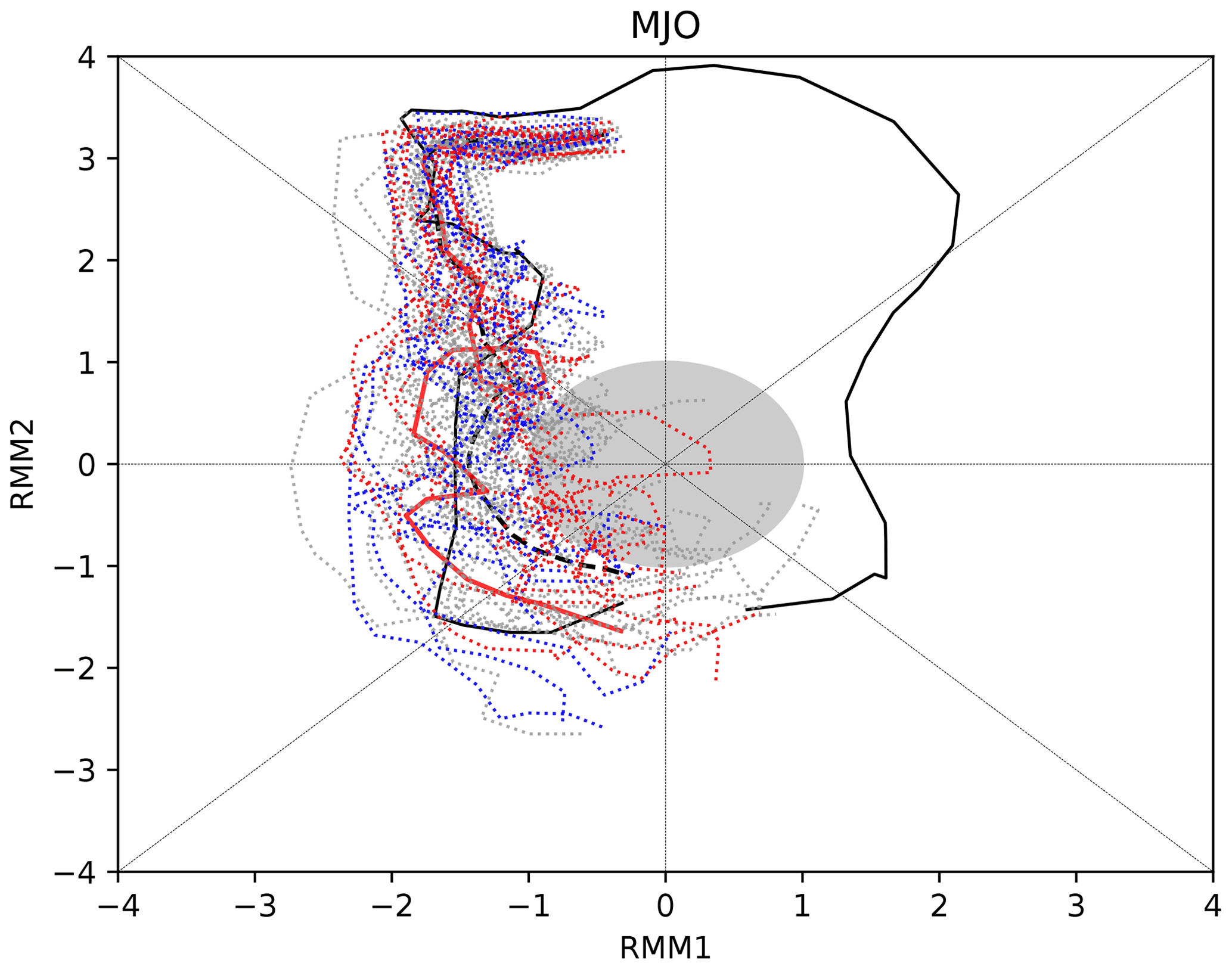
Figure A2 MJO phase diagram. ECMWF 46 d ensemble forecast initialized on 1 February: blue dashed lines denote ENS+ members, red dashed lines denote ENS− members and grey lines denote all other members (data source: http://s2sprediction.net/, last access: 23 October 2020). Red line denotes the control forecast and the black dashed line denotes the ensemble mean. Forecast data are plotted for 1–28 February. Black solid line denotes RMM indexes from the Australian Bureau of Meteorology between 15 January and 28 February 2018 (data source: http://www.bom.gov.au/climate/mjo/, last access: 23 October 2020).