the Creative Commons Attribution 4.0 License.
the Creative Commons Attribution 4.0 License.
 | 17 Jan 2024
Aquaplanet simulations with winter and summer hemispheres: model setup and circulation response to warming
Sebastian Schemm
Matthias Röthlisberger
To support further understanding of circulation changes in a warming climate, an idealised aquaplanet model setup containing summer and winter hemispheres is presented, and the results of circulation changes under warming are discussed. First, a setup is introduced that enables aquaplanet simulations with a warmer and a colder hemisphere, including realistic-looking summer and winter jet streams, storm tracks, and precipitation patterns that are fairly similar to observations, as well as a more intense and equatorward storm track in the winter compared to the summer hemisphere. The sea surface temperature (SST) distribution used here is inspired by the June–July–August zonal mean SST found in reanalysis data and is flexible to allow control of the occurrence of a single or double intertropical convergence zone (ITCZ). The setup is then used to investigate circulation changes under uniform warming, as motivated by recent research. For example, the stronger poleward shift of the storm tracks during summer compared to winter is reproduced. Furthermore, the jet waviness decreases under warming when compared on isentropes with maximum wind speed or isentropes at similar heights in pressure space. Jet stream waviness increases under warming when compared at similar-valued isentropes but primarily because the corresponding isentrope is closer to the surface in the warmer climate and waviness climatologically increases downwards in the atmosphere. A detailed analysis of the changes in wave amplitude for different wavenumbers confirms that the amplitude of large waves increases with warming, while that of short waves decreases with warming. The reduction in wave amplitude of short synoptic waves is found to dominate in the jet core region, where jet waviness also decreases and is more pronounced on the equatorward side of the jet. Long waves increase in amplitude on the poleward side of the jet and at upper stratospheric levels, which is consistent with increased jet waviness at these levels. The projected increased amplitude of planetary waves and the reduced amplitude of synoptic waves are thus clear in our aquaplanet simulations and do not require zonal asymmetries or regional warming patterns. During so-called high-amplitude wave events, there is no evidence for a preferential phase of Rossby waves of wavenumbers 5 or 7, indicating the crucial role of stationary waves forced by orography or land–sea contrast in establishing previously reported preferential phases. We confirm that feature-based block detection requires significant tuning to the warmer climate to avoid the occurrence of spurious trends. After adjustment for changes in tropopause height, the block detection used here shows no trend in the summer hemisphere and an increase in blocking in the colder hemisphere. We also confirm previous findings that the number of surface cyclones tends to decrease globally under warming and that the cyclone lifetimes become shorter, except for very long-lived cyclones.
- Article
(7285 KB) - Full-text XML
- BibTeX
- EndNote


The influence of anthropogenic climate change on atmospheric circulation and associated weather extremes has received considerable attention. For instance, weakened westerlies have been attributed to a reduction in the meridional temperature gradient due to Arctic amplification (AA; Coumou et al., 2015; Chemke and Polvani, 2020), which is particularly pronounced in the winter months. Several rather recent studies have reported summer circulation changes that are particularly concerning, as they might be associated with changes in the frequency or intensity of high-impact summertime weather and climate extremes (Coumou et al., 2015, 2018; Rousi et al., 2022). Importantly, though, for several reported summer circulation changes their magnitude and cause remain unclear or even debated, including changes in the waviness of the jet stream (e.g. Francis and Vavrus, 2012, 2015); changes in the persistence and frequency of blocked weather situations (e.g. Woollings et al., 2018) and, related to this, the preference for specific phase positions of certain wavenumber waves during high-amplitude wave events in summer (e.g. Kornhuber et al., 2020); the amplification of waves with small wavenumbers (e.g. Chemke and Ming, 2020); but also changes in the intensity, number and tracks of surface cyclones during different seasons (e.g. Priestley and Catto, 2022). CMIP simulations also suggest a stronger poleward shift in the storm tracks during summer compared to winter, except over the North Pacific (e.g. Barnes and Polvani, 2013). The seasonality of the global circulation response to warming therefore motivates simulations of lower complexity that nevertheless simulate fundamental processes that could help to explain the seasonality of the response to warming.
Regarding jet waviness, it was first suggested that weaker westerlies allow for amplified meanderings of the jet stream, causing an increase in hot and cold temperature events (Francis and Vavrus, 2012, 2015), as well as more persistent and blocked weather (Coumou et al., 2015; Francis et al., 2018). Changes in jet waviness and its causal link with regional patterns of warming such as the AA, or even just uniform warming, are, however, still “up in the air” (Francis, 2017; Cohen et al., 2019). In particular, some trends eventually result solely from incorrectly adjusting diagnostics to the warmer climate (Barnes, 2013). Indeed, idealised zonally symmetric dry simulations of polar warming (i.e. reduced meridional temperature gradients at the surface) identified a reduction in blocking frequencies and wave amplitudes and not an increase (Hassanzadeh et al., 2014). Martin (2021), however, analysed the jet waviness on the height of the jet maximum in three reanalysis products, rather than on a constant vertical height level, and identified an increase since the 1960s. Very recently, Moon et al. (2022) proposed a mechanism for an increase in the waviness of planetary waves (wavenumbers 1 to 4). In their linearised model of balanced planetary wave dynamics, which neglects synoptic baroclinic growth and prescribes a zonal asymmetric surface heat source, the planetary wave amplitude indeed increases when the vertical wind shear decreases. A further proposed theoretical underpinning of the potential trends towards more waviness and blocked and persistent weather due to wave resonance (Petoukhov et al., 2016) does not seem valid upon scrutinising the assumptions underlying the theory (Wirth, 2020; Wirth and Polster, 2021). Although wave resonance may well occur in the atmosphere if the wavenumber of free-tropospheric Rossby waves approaches the stationary wavenumber forced by topography (Charney and Eliassen, 1949), persistence of high-amplitude weather is often associated with locally recurrent Rossby wave patterns (Röthlisberger et al., 2019) rather than circumpolar wave patterns as is required by resonance (Petoukhov et al., 2016) or as found in planetary wave models (Moon et al., 2022). At the same time, however, there is evidence that large waves become less stable while small waves become more stable under warming (Chemke and Ming, 2020), and the former might indicate a larger contribution to the overall jet waviness from planetary waves. The underlying mechanism behind the “large-get-stronger, small-get-weaker” wave response to warming likely relates to the different vertical extents of large- and small-scale waves and varying trends in baroclinicity at different vertical levels in the atmosphere (Rivière, 2011). Indeed, Martin (2021) suggested that the upwards trend in waviness identified in three reanalysis products may not result from Arctic amplification (and reduced vertical wind shear; Moon et al., 2022) but from an increase in the frequency of anticyclonically tilted waves at the jet stream level that have larger length scales than cyclonically tilted waves (Rivière, 2011), which seems consistent with the large-get-stronger, small-get-weaker wave response.
The climatic situation is complicated because regional trends may oppose each other; for example, Francis et al. (2018) identified an increase in the persistence of weather regimes over North America, while Huguenin et al. (2020) found no trend in persistence in circulation regimes over Central Europe (neither in summer nor in winter). Consistent with that, globally, the trend in the frequency of blocking is not yet conclusive (Woollings et al., 2018). Regional persistence trends over Europe can be reconciled with the projected poleward shift and eastwards extension trend of the North Atlantic storm track (Kyselý and Domonkos, 2006; Hoskins and Woollings, 2015; Harvey et al., 2020) and thus can be considered only as passive changes and not as a global reduction in blocks. From this projected storm track shift, one can also expect a regional reduction in the number of surface cyclones over Europe. However, the number of surface cyclones appears to decrease globally during summer (Zappa et al., 2013; Chang et al., 2016) and winter (Priestley and Catto, 2022). For surface cyclones, there is some evidence from previous wintertime idealised warming experiments with atmospheric general circulation models (AGCMs) that the number of cyclones decreases globally even under simple warming (Sinclair et al., 2020; Schemm et al., 2022), and the reduction in the number of cyclones hence appears to be the most robust of the above-discussed changes.
As expected when considering these topics, the variety of methods to detect blocks, cyclones, waviness, weather regimes or persistence is so large that the observed trends are not always clear (Kučerová et al., 2016). More so, studies have questioned whether weather regimes defined by statistical cluster techniques are regimes that are per se more persistent in the sense of the slowly evolving trajectory of the system within a phase space (Fereday, 2017). Uncertainties in cyclone track statistics arise from various cyclone tracking methods (Neu et al., 2013). Uncertainties in trends of jet waviness may result from the fuzzy concept of waviness in general and the application of different methods to different height levels (Barnes, 2013). For example, Martin (2021) employs a geometric definition of jet waviness and applies it to the height of the maximum wind speed. Hence, the height level changes at each time step and follows the jet core. The finding is an upwards trend in waviness since the 1960s. Blackport and Screen (2020) use a related method but report no clear upwards trend. Eventually, the difference is because their study is based on a different height level (i.e. 500 hPa), which is held constant over time but under warming changes its height above the surface. The exact cause of the often contrasting results remains unclear.
A conclusion that emerges from the above overview is that idealised studies of summertime and wintertime circulation changes are potentially a useful stepping stone of intermediate complexity to (a) establish a baseline response of the summertime circulation to simple warming, (b) explore the need to adapt feature-based detection methods to a warmer climate and (c) make the data available for the community to explore the performance of various further diagnostics. Toward this end, we propose an idealised aquaplanet setup that comprises a warmer summer-like and colder winter-like hemisphere shaped exclusively by the underlying sea surface temperature (SST) distribution. In the warmer hemisphere, the Equator-to-pole SST gradient is weaker than that in the colder hemisphere, favouring the development of weaker summer-like jet streams and storm tracks that are as in observations located further poleward compared to winter. Furthermore, similar to the boreal summer observations, the maximum SST values are shifted into the warmer hemisphere, and the cross-equatorial SST gradient can be used to control the occurrence of a single or double Intertropical Convergence Zone (ITCZ) (Bischoff and Schneider, 2016; Adam et al., 2016). Such a hemispheric asymmetric SST distribution, which can be used for the simulation of a summertime aquaplanet, is potentially also useful for a variety of further research questions related to circulation changes in a warmer climate or serves as a test case for numerical model development. To the best of our knowledge, no summertime aquaplanet experiments (APEs) have been systematically studied thus far.
This study therefore consists of two main parts. In the first part, we introduce the setup, design and mean climatologies of an aquaplanet simulation with winter and summer hemispheres. In the second part, we demonstrate the usefulness of our APE setup by going through the above-discussed summer circulation changes and by testing their existence in our APE simulations. Specifically, we address the following questions:
-
How does jet waviness change under simple uniform warming, and what is the role of changes in the height of the investigated isentropic level (e.g. Barnes, 2013; Francis and Vavrus, 2015)?
-
Is a large-get-stronger, small-get-weaker wave response to warming (e.g. Chemke and Ming, 2020) apparent in APE simulations, and at which altitude do the changes occur?
-
Is there a preferred phasing of high-amplitude large-scale waves even in the absence of zonal asymmetries in the mean state (Kornhuber et al., 2020)?
-
How is the global frequency of atmospheric blocking affected by uniform warming (e.g. Woollings et al., 2018)?
-
How does the frequency of surface cyclones change globally in a simple warming experiment (e.g. Priestley and Catto, 2022)?
Importantly, we cannot expect a summertime-like APE to reproduce all observed and simulated summer circulation changes found in fully coupled GCMs, which include an interactive ocean and topography. Rather, the presence of some changes and the absence of others may indicate the relative importance of components that were not considered in the APE setup. Here, we thus use an APE setup for constraining the palette of possible causes of circulation changes, e.g. for ruling out or emphasising the importance of changes in zonal asymmetries such as land–ocean contrasts, the AA, changes in ocean circulation or topography as causes for circulation changes simulated by Earth system models (ESMs).
2.1 Jet waviness
To quantify the waviness of the jet stream, we use the geometric definition of waviness as in Röthlisberger et al. (2016) and Martin (2021). The jet stream axis is defined as the 2 PVU contour on an isentropic surface. The absolute value of the latitude difference between adjacent points along the contour is summed. This geometric definition of waviness follows the proposal of Röthlisberger et al. (2016), who related this type of waviness measure to the occurrence of extreme surface weather where the type of extreme occurrence (i.e. wind, precipitation, or temperature) associated with high waviness is shown to vary regionally. A zero waviness indicates a pure zonal flow, and there is no maximum in the definition of this waviness, similar to the method of Martin (2021). At times, several closed 2 PVU contours are detected, for example, in the presence of additional potential vorticity (PV) cut-offs. In this case, the algorithm selects the longest contour for computing the waviness. Following suggestions from previous studies (Barnes, 2013; Martin, 2021), we quantify jet waviness changes in three different ways: (1) we compare jet waviness on the same isentrope between a control and a warmed simulation; (2) we compare jet waviness on two different isentropes, which, however, in the zonal mean are both at the same pressure level; and (3) for each time step and in both simulations, we choose the isentrope for which the maximum wind speed is found.
2.2 Rossby wave amplitudes
To further examine changes in Rossby wave dynamics under uniform warming, we also perform analyses inspired by Chemke and Ming (2020). In particular, for all simulation setups, we compute the Fourier transform of the meridional wind (v) over longitude for each 6-hourly time step t at each pressure level p and latitude ϕ. Then, we compute the amplitude of the waves for each wavenumber k as the modulus of the respective Fourier coefficient, i.e. , whereby is the respective coefficient for wavenumber k. Finally, we compare the wave amplitudes between the warmed and control simulations by computing the amplitude difference:
where the overline denotes the time mean. Due to the rise in tropopause height as well as vertically differing changes in baroclinicity expected under warming (e.g. Rivière, 2011; Barnes, 2013), we are particularly interested in the vertical structure of the Rossby wave amplitude changes.
2.3 Rossby wave phases
To examine the existence of a preferred phasing of high-amplitude waves, we repeat and slightly expand the analyses of Kornhuber et al. (2020) for our simulations. We first compute Hovmöller diagrams of the 7 d averaged 300 hPa meridional wind, averaged between 35 and 65∘ latitude of the respective hemisphere (hereafter denoted as vhov(λ,t), whereby λ is longitude). A Fourier transform over longitude is then also applied to vhov(λ,t), and the resulting (complex) Fourier coefficients for wavenumbers 5–8 (νhov(k,t)) are used to examine a preferred phasing of high-amplitude waves. Specifically, we again compute the amplitude of each of these wavenumber waves for each week as . Then, the phase Φhov,k(t) (in radians from −π to π) is computed as
where arctan2 is the two-argument arctangent. As in Kornhuber et al. (2020), we then compute for wavenumbers 5–8 the standard deviation σhov,k of Ahov,k(t) and define weeks with “high-amplitude waves” as weeks for which . For the roughly forty seasons per simulation setup, this yields between 36 and 48 weeks with high-amplitude waves per wavenumber (compared to 44–47 in Kornhuber et al., 2020, for an equally long data record). The number of weeks with high-amplitude waves in a specific wavenumber is hereafter referred to as Nk.
To examine whether there is a statistically significant preference for particular phases during the high-amplitude weeks of any of the wavenumbers, we extend the analysis of Kornhuber et al. (2020) with a bootstrapping test. We first compute a histogram of the Φhov,k(t) values for each wavenumber with eight bins of width . Then, we randomly select 10 000 times Nk weeks. For these sets of Nk weeks, we again compute histograms of the respective Φhov,k(t) values. Here, we identify a statistically significant preferred phasing when the count of the actual high-amplitude Φhov,k(t) values in one bin of the histogram lies outside the 2.5 to 97.5 percentiles of the respective counts of the randomly generated histograms.
2.4 Blocks
The identification of atmospheric blocks is based on persistent, vertically averaged, upper-tropospheric potential vorticity (VAPV) anomalies (Schwierz et al., 2004; Croci-Maspoli et al., 2007; Sprenger et al., 2017). Specifically, a northern hemispheric block is identified as a coherent area with a negative VAPV anomaly of less than −1.0 PVU () and persisting for at least 5 d. Note that the commonly used threshold of −1.3 PVU (e.g. Croci-Maspoli et al., 2007) is not suitable for blocking identification in summer. To allow for the detection of summertime blocks, the less restrictive threshold of −1.0 PVU is used here, as in Röthlisberger and Martius (2019). Likewise, in the Southern Hemisphere, where potential vorticity is generally negative, a VAPV anomaly is required to be in excess of 1 PVU.
In a basic configuration of the blocking identification, vertical averages are computed for the layer between 500 and 150 hPa. These averages are hereafter referred to as VAPV0. Because changes in the tropopause height, as evidenced by the warmed simulation results (see Fig. 5), can profoundly influence the climatology of VAPV and the strength of VAPV anomalies (Croci-Maspoli et al., 2007), blocking identification in the warmed simulations is additionally performed with vertically shifted layers. Three additional layers are considered: layers shifted by 25 and 50 hPa upwards, VAPV25 (475–125 hPa) and VAPV50 (450–100 hPa), respectively, and an adjusted VAPVA defined as the mean of VAPV0 and VAPV25.
The model output of PV is available at pressure levels in intervals of 25 hPa. Climatological and hemispheric (poleward of 30∘ N or 30∘ S) averages of VAPV25 and VAPV50 in the warmed simulations do not closely match VAPV0 in the control simulation. In contrast, the differences between climatological and hemispheric averages of VAPVA in the warmed simulations and VAPV0 in the control simulations are reasonably small.
2.5 Cyclones
The diagnostics introduced above are complemented by feature-based identification of cyclones. Surface cyclone detection is based on the sea-level pressure (SLP) contour search approach by Wernli and Schwierz (2006) and refined for merging and splitting cases following Sprenger et al. (2017). Minima in SLP are accepted as cyclones if enclosed by an SLP contour and traceable for at least 24 h in 6-hourly data. Grid points inside the outermost closed SLP contour are flagged with ones, with all other grid points with zero yielding cyclone masks that are used to compute cyclone frequencies. Cyclone frequencies correspond to the percentage of time steps that a grid point is affected by a cyclone mask. Deepening rates are calculated based on 6-hourly SLP changes along the SLP minimum of a track, and genesis and lysis are defined as the first and last time steps along a track, respectively. The total number of cyclone tracks is approximately 35,000 tracks in the control simulations and 32 000 in the warmed simulations. Most cyclone detection schemes agree on the tracks and existence of deep systems, while there is larger uncertainty related to the exact location of cyclogenesis, lysis, and tracks for shallow and short-lived systems (Neu et al., 2013; Walker et al., 2020; Roebber et al., 2023). For the purpose of our study, the exact track and genesis or lysis locations are not relevant, and the changes in the number of tracks are qualitatively compared to previous studies using different detection methods (Sinclair et al., 2020).
All five of the diagnostics introduced above have been used in previous reports and are applied here to data that are interpolated across a 1∘ by 1∘ grid with a 6 h temporal resolution.
APEs are numerical modelling simulations in which the entire surface of the Earth is covered by water, which sometimes features additional zonal asymmetries. Examples include warm or cold sea surface temperature (SST) anomalies (Brayshaw et al., 2008; Sampe et al., 2013; Schemm et al., 2022) and SST gradient changes (Brayshaw et al., 2011a; Williamson et al., 2013) or idealised topography and continents (Brayshaw et al., 2011a). Including zonal surface asymmetry in an APE allows reproducing the triple pattern of change seen in CMIP future projections of the North Atlantic storm track, which does not occur in zonally symmetric APEs (Schemm et al., 2022). Furthermore, APEs are frequently used to test new numerical schemes or model grids and have established themselves as a standard test for model intercomparison studies (Blackburn et al., 2013), including studies focusing on tropical dynamics (Nakajima et al., 2013). Most APE simulations are inspired by the boreal wintertime climate. Below, we propose a setup that has a summer and a winter hemisphere at least in its SSTs.
3.1 The generalised “Qobs” SST distribution
At the core of an aquaplanet simulation is the SST distribution. In the absence of an interactive ocean and land surface, the SST distribution shapes the global asymmetries in near-surface temperature and thus the location of the major baroclinic zones, the strength of the jet stream, and the position and shape of the ITCZ. Most APE studies rely on the symmetric distribution of sea surface temperature (SST) originally proposed by Neale and Hoskins (2000) and known as “Qobs”, or the slightly extended version of it as defined in Brayshaw et al. (2011b) and known as “Qobswide”. Both designs follow the zonal mean SST of the Northern Hemisphere (NH) from December to February (DJF). The zonal mean SST of the NH is mirrored in the Southern Hemisphere (SH) to obtain a symmetric SST distribution with a peak, where the peak is located at the Equator. Radiation is typically set to the solar equinox. In this way, both hemispheres are established with initial conditions that are perfectly symmetric with respect to the radiation and SST distributions and can be considered one long time series, namely an NH winter-like series, which is a computationally attractive design to obtain a perpetual winter.
The SST distribution in this study is based on a generalised form of the established “Qobs” distribution of Neale and Hoskins (2000), which allows us to mimic a summer and winter hemisphere. We define the generalised “Qobs” SST distribution as follows:
where w1 is a weighting parameter, Tmelt is the freezing temperature of water, Tmax is the maximum SST (Tsst, Tmelt and Tmax have units of ∘C) and the latitudinal variation f(ϕ) is modelled in each hemisphere by
where ϕ0 is the latitude where the SST distribution becomes zero (Tmelt) and ϕmax is the latitude where the SST distribution reaches its maximum (Tmax; here set to 28 ∘C). The transition between a single and double ITCZ is controlled by the weighting parameter w1. The occurrence of the transition for a given weighting parameter is highly model-dependent, and the proposed SST distribution can thus be used in future intermodel comparison studies. The parameters can be used to fit the SST distribution to, for example, zonal mean reanalysis data.
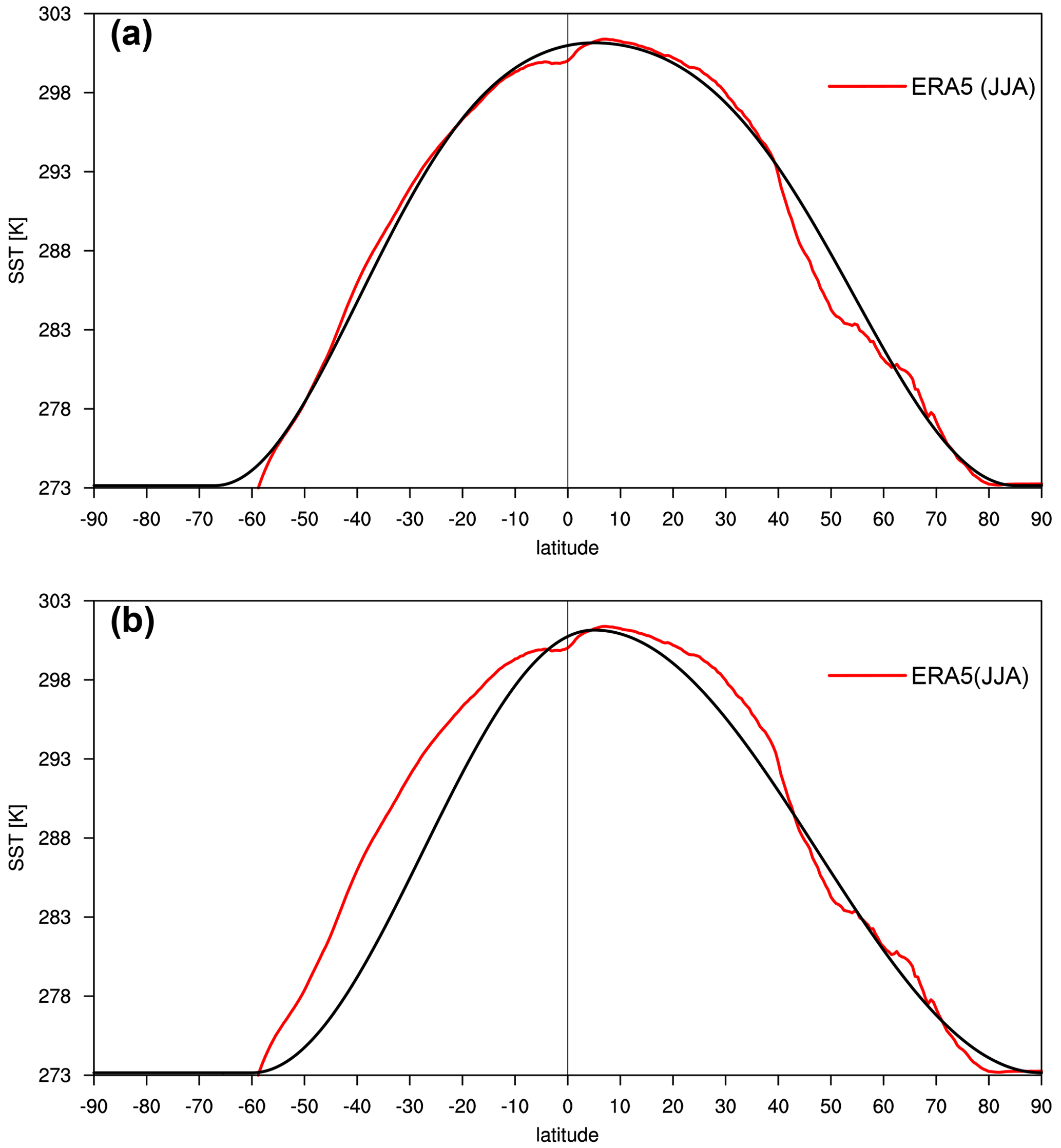
We use two weighting parameters to measure the sensitivity of the results to the shape of the SST. First, we fit the generalised “Qobs” distribution to the June–July–August (JJA) zonal mean SST distribution obtained from ERA5 using w1=0.5, and in the colder and in the warmer hemisphere (Fig. 1a). Second, we choose a steeper SST distribution (w1=1) that also peaks in the warmer hemisphere at 5∘ N. Because the observed SST distribution during JJA approaches Tmelt at lower latitudes in the winter hemisphere, we set in the colder hemisphere and in the warmer hemisphere (Fig. 1b). As shown below, the first SST distribution results in the formation of a double ITCZ, while the latter results in the formation of a single ITCZ.
3.2 Model setup and mean climate
ICON model and initial conditions. The idealised experiments in this study are performed with the nonhydrostatic weather and climate prediction model ICON (Zängl et al., 2014) in version 2.6.5. The equivalent grid spacing of the icosahedrical grid is approximately 80 km, and the time step is 360 s. The model top is at 65 km and spanned by 70 vertical levels using the SLEVE coordinate system (Schär et al., 2002). The vertical layer thickness is 20 m near the surface and increases to approximately 200 m at an altitude of 1.5 km, 500 m at an altitude of 8 km, 1000 m at an altitude of 20 km and 3000 m at an altitude of 60 km. The subgrid-scale parameterisations include the ecRad radiation scheme developed at ECMWF (Hogand and Bozzo, 2018), and radiation is computed on a horizontal grid that is reduced in space by a factor of 2 and is updated at every second time step. Furthermore, a one-moment two-category microphysics scheme (Doms et al., 2011), a deep convection parameterisation Tiedtke (1989) and a turbulent transfer subgrid-scale model based on (Doms et al., 2011) were used. Finally, non-orographic gravity wave drag is parameterised following Orr et al. (2010). This set of subgrid-scale parameterisation and initial conditions is similar to that in Schemm et al. (2022). The model is initialised with temperature, pressure and wind according to Jablonowski and Williamson (2006) and simulates 10 years, resulting in 40 seasons with summer-like SSTs in the NH and 40 seasons with winter-like SSTs in the SH.
Radiation. In a setup with fixed SSTs and no land surface, radiation has little effect on the climatological mean surface temperatures, and as in most aquaplanet experiments, the solar zenith angle is set to a perpetual equinox. Thus, both hemispheres receive the same radiation. The climatological differences between the two hemispheres in turn originate from only the SST distribution. Indeed, when we repeat the simulations with the radiation fixed to the summer solstice in the NH, the effect of the changed solar orbital on the mean climate of the aquaplanet is negligible. For simulations with land surfaces, setting the radiation to the solstice in the warmer hemisphere is crucial to obtain realistic winter and summer hemispheres, but in the setup used here with fixed SST radiation, surface temperatures cannot be changed.
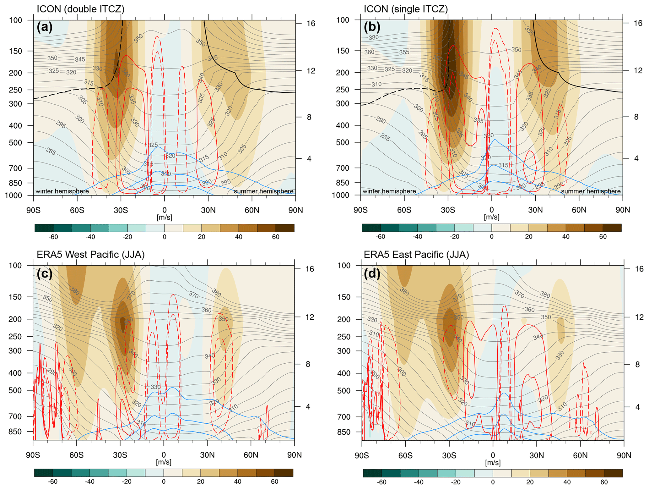
Figure 2Vertical cross section (left axis pressure: hPa; right axis height: km) of zonal mean zonal wind (shading; m s−1), potential temperature (grey contour; in steps of 5 K), vertical motion (red contours; upwards dashed and downwards solid; ±0.4 and 0.8 hPa h−1) and specific humidity (blue contours; 3, 7 and 11 g kg−1) for ICON aquaplanet simulations with (a) the flat and (b) the steep SST distributions shown in Fig. 1. (c, d) Similar to (a) and (b) but for ERA5 averaged across the (c) West Pacific (160–180∘ E) and (d) East Pacific (120–180∘ W) during JJA. Additionally, shown in (a) and (b) is the dynamical tropopause (dashed and solid black; ±2 PVU).
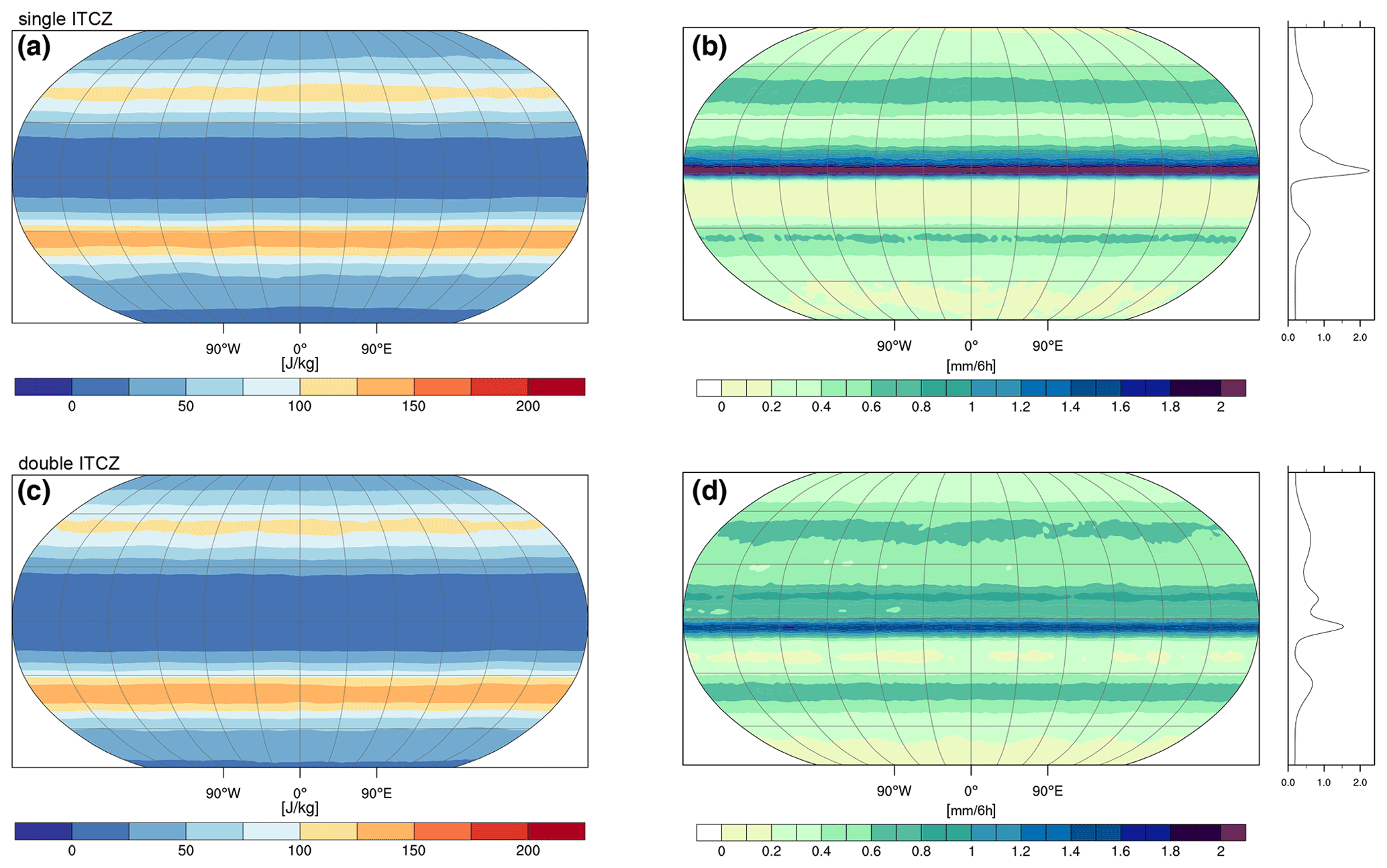
Figure 3(a, c) The 10 d high-pass-filtered eddy kinetic energy (EKE; J kg−1) vertically averaged between 100–850 hPa for (a) the single- and (c) the double-ITCZ base states. (b, d) The 6-hourly accumulated precipitation (shading; kg m−2) for (b) the single- and (d) the double-ITCZ base states.
Mean climate. The zonal average of selected variables for the ICON simulation and ERA5 (JJA; 1979–2022) is shown in Fig. 2. Figure 2a corresponds to the mean climate based on the flatter SST distribution depicted in Fig. 1a. The midlatitude jet is, as in reanalysis data, weaker in the summer hemisphere and located farther poleward than the stronger jet in the wintertime hemisphere. The vertical motion indicates the development of a double ITCZ, with the stronger branch near the Equator and the weaker branch at 10∘ N. Thus, the maximum ascent flanks the maximum SSTs located at 5∘ N. The descending subtropical branch is stronger in the colder hemisphere, and a well-developed region of ascent at 45∘ S indicates the existence of a storm track that is more intense in the colder SH than in the summer NH, which is also seen in vertically averaged eddy kinetic energy (Fig. 3), broadly consistent with reanalysis data. A double ITCZ is a feature observed in the reanalysis data, for example, over the western Pacific (Fig. 2c). The second, steeper SST distribution (Fig. 1b) results in the formation of a single ITCZ (Fig. 2b), as is observed, for example, over the eastern Pacific (Fig. 2d). In the single-ITCZ case, a single precipitation peak emerges north of the Equator in the warmer hemisphere, while in the double-ITCZ case, the precipitation peak in the warmer hemisphere is reduced, and a second and stronger precipitation peak emerges slightly south of the Equator (Fig. 3b, d), which agrees with patterns of vertical motion (Fig. 2a). Precipitation peaks are flanked by two descending subtropical branches, both of which are characterised by nearly zero precipitation in the winter hemisphere, with more precipitation in the warmer hemisphere (see zonal mean next to Fig. 3b, d). The jet streams are stronger in both hemispheres compared to the flat SST case, as expected due to the locally larger meridional SST gradients. The winter jet reaches up to 60 m s−1 (Fig. 2a, b), which is stronger than in the reanalysis data.
Overall, the asymmetric SSTs result in a summer and winter hemisphere with realistic large-scale flow features such as midlatitude jets, storm tracks and precipitation patterns. Because a double and a single ITCZ are both observed in reanalysis data (albeit at different longitudes), both SST configurations are used hereafter to examine the response of the circulation in the summer hemisphere to a uniform 4 K warming of both SST configurations.
4.1 Poleward storm track shift
CMIP models project a poleward shift in storm tracks under warming at the end of the century, which is particularly pronounced in the SH (Chang et al., 2012; Barnes and Polvani, 2013; Priestley and Catto, 2022). There is a seasonal and basin dependence in the extent to which storm tracks shift poleward. In the SH, the poleward shift is stronger during summer (DJF; avg. of 2.2∘ poleward) than during winter (JJA; avg. of 1.8∘ poleward) (see Fig. 12 in Barnes and Polvani, 2013). The North Atlantic winter storm track exhibits only a weak poleward shift (Woollings et al., 2012), but the shift is well-marked during summer (Barnes and Polvani, 2013). The North Pacific behaves differently; it shifts poleward, particularly during the cold season and much less during the warm season, which might be related to the seasonal variability and interaction with the subtropical jet (see Fig. 12 in Barnes and Polvani, 2013). In general, the polar shift is strongest in autumn in the North Atlantic and SH, but the increased shift in summer (compared to winter) motivates a brief investigation of this effect as predicted by our aquaplanet setup.
The change in latitude of the maximum in zonally and vertically averaged EKE between 700 and 100 hPa is used to quantify the storm track shift. Indeed, in the colder hemisphere and in the double (single) ITCZ simulation, the latitude shift is 2∘ (2∘) poleward, while it is 4∘ (3∘) in the warmer hemisphere. This larger poleward shift in the warmer hemisphere is in agreement with the SH and North Atlantic storm track shifts seen in CMIP data. Barnes and Polvani (2013) used low-level averaged zonal winds to investigate the poleward shift. The motivation for the low-level averaged wind field is that it allows the separation of the deep eddy-driven jet from the more upper-level shallow subtropical jet. When analysing low-level wind, we find in the colder hemisphere with a single (double) ITCZ, the shift is 2∘ (1∘) poleward, while it is 3∘ (3∘) in the warmer hemisphere. Thus, there is a tendency for the aquaplanet setup presented here to reproduce the seasonality of the poleward shift in the storm track in more comprehensive Earth system model simulations, which is better seen in EKE. The setup can therefore be used to further investigate the mechanisms underlying the more pronounced shift in summer compared to winter, seen in the SH and North Atlantic, while the aquaplanet does not reproduce the seasonal dependency of the North Pacific storm track.
4.2 Jet stream waviness
First, we note that the climatological waviness varies vertically and increases towards the surface (Fig. 4a), reflecting the fact that the jet becomes more zonal at upper levels. For example, in the single-ITCZ run, the median jet waviness decreases in the summer hemisphere by approximately 12 % when moving from 330 to 340 K. The reduction with height is on a similar order of magnitude for the winter hemisphere, although the waviness is generally smaller in the winter hemisphere by approximately 40 % at 330 and 340 K (not shown).
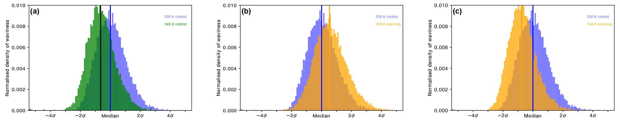
Figure 4Normalised histograms of 6-hourly jet stream waviness for the summer hemisphere for (a) 330 (blue) and 340 K (green) in the control simulation, (b) 330 K in the control (blue) and warmed (orange) simulations, and (c) 330 K in the control (blue) and 340 K in the warmed (orange) simulations in the single-ITCZ run. Vertical lines indicate the median of the respective distributions. The normalisation is done so that the integral over all bins is one.
Next, we examine waviness changes between warmed and control simulations. When comparing the jet waviness on similar isentropic surfaces in the summer hemisphere, we find an increase in jet waviness, for example, at 330 K (Fig. 4b). In this case, the distribution of the jet waviness in the warmed simulation is shifted towards higher values by approximately half a standard deviation of the control run and consequently reaches higher extreme values (yellow in Fig. 4b). This comparison indicates that the jet waviness increases in a warmer climate, but the change is on the same order as the change we observe when comparing waviness on the 330 and 340 K surfaces in the control run. Hence, if jet waviness is compared on a constant isentropic surface, changes in the height of that surface due to warming may introduce a spurious trend in jet waviness due to the climatologically decreasing jet waviness with height. This trend result agrees with the findings of Barnes (2013).
A contrasting picture emerges when jet waviness is compared between two isentropic surfaces that are on the same height in pressure space in the zonal mean of the control and warmed simulations. Figure 5 shows the height of the 320, 330 and 340 K isentropic surfaces in the control and warmed simulations. For example, the height of the 330 K surface in the control simulation corresponds well to the 340 K surface in the warmed simulation, and the same is true for the 320 and 330 K surfaces. While the slope of the isentropes does not change at mid-latitudes, the changes in altitude in response to a 4 K surface warming lead to a match in height between isentropic surfaces that are 10 K apart. Note that for very high surfaces, such as 350 K, the upwards expansion of diabatic heating in the tropics causes the isosurface to bend downwards in the warmed simulation, while it bends upwards in the control simulation. Comparing jet waviness on the 330 and 340 K surfaces, the distribution of the warmed simulation is shifted towards lower values compared to the control simulation (Fig. 4c), and the conclusion is that the jet waviness decreases in the warmer simulation, which is to say that, by adjusting the isentropic level, the trend reverses.
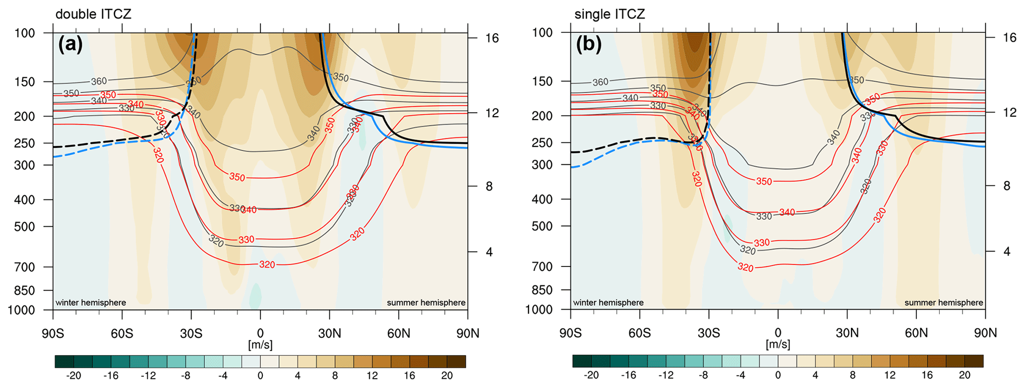
Figure 5Vertical cross section (left axis pressure: hPa; right axis height: km) of zonal mean difference between control and simulation warmed at the surface by +4 K for the (a) double and (b) single-ITCZ simulation. Shown are differences in zonal wind (shading; m s−1), selected isentropic surfaces (red warmed and grey control simulation) and the dynamical tropopause (blue control and black warmed simulation).
Finally, as in Martin (2021), we compute the jet waviness at each 6-hourly time step on the isentrope with maximum wind speed and find a systematic shift towards reduced waviness (Appendix Fig. A2). The median values computed based on the 6-hourly time series of isentropes with maximum wind speed are 333.4 K for the control simulation with a single ITCZ and 344.2 K for the corresponding warmed simulation. The above comparison of the jet waviness between 330 and 340 K is thus reasonable, as both are close to the mean isentrope that carries the maximum wind speed. The increase in jet waviness found by Martin (2021) is thus not reproduced in the zonally uniform APE with uniform warming, at least not on the summer hemispheric side of the APE.
In the colder hemisphere, the dynamics are more complex. Accounting for the change in altitude, the jet waviness at 320 K is best according to the climatological zonal mean compared to 330 K in the warmer simulation. The jet waviness also decreases (Fig. A1a). Further above, however, when comparing 330 to 340 K, we find similar distributions of the jet waviness (not shown). Even further above, for the 340 K control compared to the 350 K warmed case, we find an increase in jet waviness (Fig. A1b). Accordingly, jet waviness at this level appears to increase but not due to a change in the altitude of the isentropes. We return to this result after discussing changes in the amplitude of small and large waves in the next section.
We also note that in the above section, consideration was given to the changes in jet waviness in the single-ITCZ simulation. Qualitatively, the results are similar for the double-ITCZ run. The results are thus insensitive to this aspect of the mean state of the model.
4.3 Changes in Rossby wave amplitudes
In this subsection, we further examine Rossby wave characteristics in our simulations by considering the changing amplitudes of different wavenumber waves. Hereby, we specifically examine whether the large-get-stronger, small-get-weaker wave response to warming (Chemke and Ming, 2020) is apparent in our simulations. Figure 6 shows the climatological amplitudes Ak(p,ϕ) as well as amplitude differences ΔAk(p,ϕ) for wavenumbers and 9 for both the single (a, c, e, g) and double (b, d, f, h) ITCZ setups (results for wavenumbers and 10 are qualitatively similar; not shown). Evidently, the response to uniform warming differs considerably between large waves () and synoptic wavenumber waves () but is qualitatively very similar between the single- and double-ITCZ setups. In the summer hemisphere, the wavenumbers 3 and 5 feature the largest amplitudes poleward of the jet and amplify under warming. However, this amplification is largely constrained to levels above 300 hPa and, moreover, is largest at the poleward and equatorward edges of the jet. This increase in wave amplitude does not project to an increase in jet waviness at the jet axis (as shown in the previous section), likely because it occurs away from the jet axis and is offset by the decrease in the wave amplitude of short waves. The increase in the amplitude of large waves thus essentially constitutes an upwards extension of the regions with the largest wave 3 and 5 amplitudes. In stark contrast, the region of maximum amplitude of waves 7 and 9 is located close to the jet maximum in the summer hemisphere, and the ΔA7(p,ϕ) and ΔA9(p,ϕ) fields reveal a decrease in wave amplitude below the jet maximum as well as on its equatorward side. At the same time, a weak increase in the amplitudes of these wavenumber waves is discernible above 200 hPa, particularly on the poleward side of the jet.
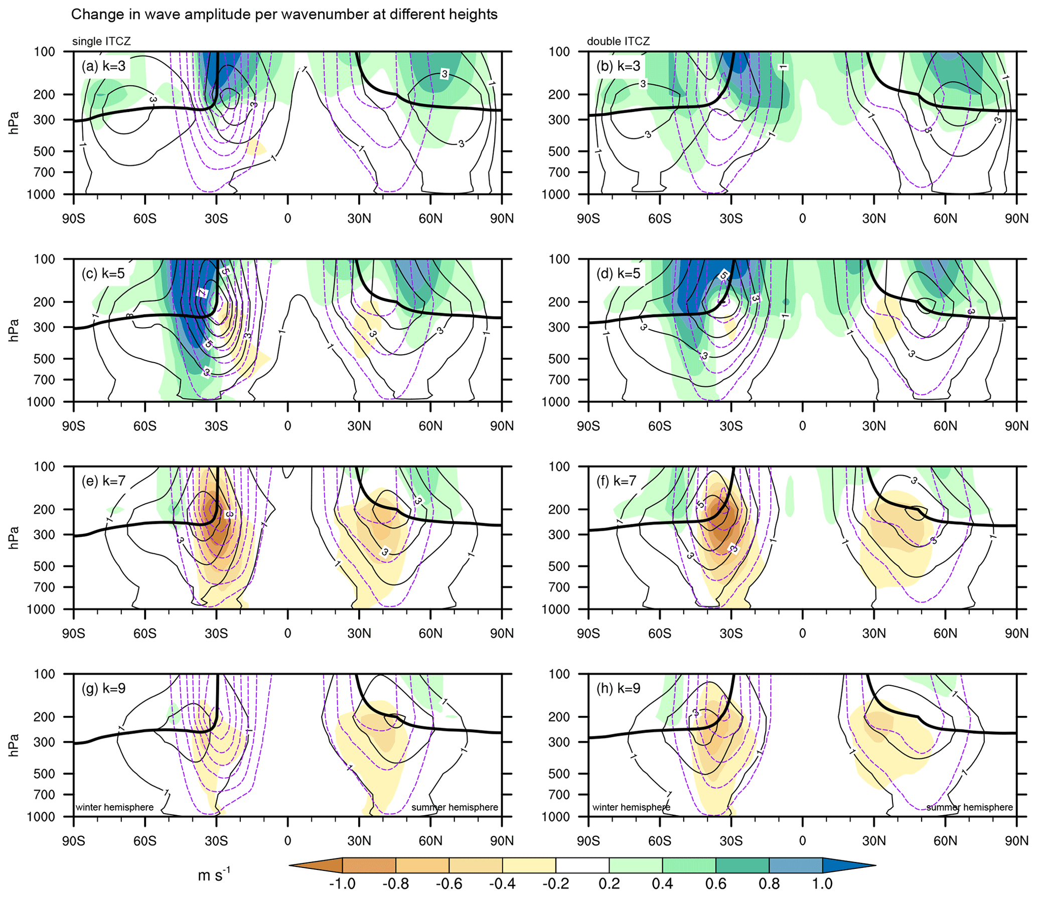
Figure 6Shading depicts amplitude differences ΔAk(p,ϕ) for and 9 waves in (a, c, e, g) the single-ITCZ and (b, d, f, h) the double-ITCZ runs, respectively. Light black contours show the (time-averaged) amplitudes Ak(p,ϕ) of the control simulation for the respective wavenumbers with a contour spacing of 1 m s−1. Dashed purple and solid black contours show the zonal wind (starting at 10 m s−1, in 10 m s−1 steps) and the zonal mean 2 PVU line, respectively.
The changes in wave amplitudes in our APE indeed reveal a large-get-stronger, small-get-weaker wave response to warming and are thus consistent with the results of previous studies assessing such changes in far more complex global warming simulations (Rivière, 2011; Chemke and Ming, 2020). One possible explanation for this response is that large waves are much less confined to lower levels than small waves and therefore benefit from an increase in upper-level baroclinicity, whereas an increase in low-level baroclinicity would benefit the growth of both small and large waves (Rivière, 2011). Closer inspection of changes in the Eady growth rate indeed shows an increase at 20–30∘ N/S between 250–100 hPa (though not shown, note the steeper isentropic slope in this region in Fig. 5), consistent with a prior report by Rivière (2011). However, given that in many parts of the free troposphere, baroclinicity changes little in our simulations, the mechanism underlying the reduction in the amplitude of synoptic wavenumber waves in the free troposphere remains unclear.
As mentioned, the increase in wave amplitude of large waves seems not to be reflected in an increase in jet waviness. However, there is one exception. The increase in the amplitude in the colder hemisphere for wavenumber 5 (blue shading in Fig. 6c) is strongest close to where an increase in the waviness of the jet was observed at very high isentropes (350 K). While in general, changes in all wavenumbers collectively drive the waviness of isentropic 2 PVU contours (indicative of the jet geometry), in this sector, the response seems to be dominated by changes in wavenumber 5 (and less), while elsewhere, it is dominated by the decrease in amplitude (and hence jet waviness) of wavenumber 7 (and larger). The changes in the wavenumbers that dominate the signal at different levels are all in agreement with the previously reported waviness changes. While those in the core are dominated by synoptic wavenumbers, there is apparently also an increase in planetary wave amplitude and jet waviness that occurs in the absence of zonal asymmetries (and AA), which is a key requirement for the mechanism described in the model of Moon et al. (2022). Additionally, from the above, it follows that synoptic baroclinic waves and changes in their amplitude dominate at the jet stream level and thus cannot be neglected.
In summary, Fig. 6 clearly reveals that the large-get-stronger, small-get-weaker wave response to warming is apparent in our APE simulations. This outcome suggests that this response, which was first diagnosed in fully coupled GCMs, may be unrelated to changes in zonal asymmetries, such as the land–ocean contrast, but rather arises due to changes that are reproduced in our simulations, such as changes in free-tropospheric and upper-level baroclinicity. Furthermore, Fig. 6 further underlines that changes in wave amplitudes not only are scale-dependent (Chemke and Ming, 2020) but also vary between altitudes as well as latitudinally, even in the absence of zonal asymmetries. Moreover, on different levels, the changes in wave amplitude can be reconciled with changes in jet waviness. However, in the jet core, synoptic wavenumbers dominate the changes.
4.4 Preferred phasing of high-amplitude waves
Recently, Kornhuber et al. (2020) found that in Northern Hemisphere summer quasistationary, synoptic wavenumber waves exhibit a preferred phasing that fosters concurrent heat waves in major breadbasket regions, particularly central North America, western Europe and western Asia. Such slow-moving amplified hemispheric wave patterns have been observed during the concurring weather extremes in early summer 2018 (Kornhuber et al., 2019), and their increasingly frequent occurrence has been suggested as a potential cause of the significantly larger trends in heat waves in western Europe compared to other regions (Rousi et al., 2022). For planetary-scale stationary waves, i.e. , it is well understood that they have a preferred phasing set by quasistationary forcing mechanisms, such as land–ocean contrasts, topography or slowly evolving sea surface temperature anomalies (e.g. Hoskins and Woollings, 2015). However, for synoptic wavenumber (k>4) waves, the causes of a preferred phasing of high-amplitude waves are far less clear, as these waves are typically considered to be transient. Previously formulated hypotheses based on the notion of quasi-resonant amplification (e.g. Petoukhov et al., 2016) offer significant shortcomings on a theoretical level (Wirth, 2020; Wirth and Polster, 2021), and other explanations for this phenomenon, such as the notion of recurrent Rossby waves (Röthlisberger et al., 2019), remain rather observational. To narrow the possible causes of a preferred phasing of high-amplitude synoptic waves, we thus assess whether a preferred phasing is apparent in any of our APE simulations, with the hypothesis that no preferred phasing occurs due to the zonally symmetric setup of the APE.
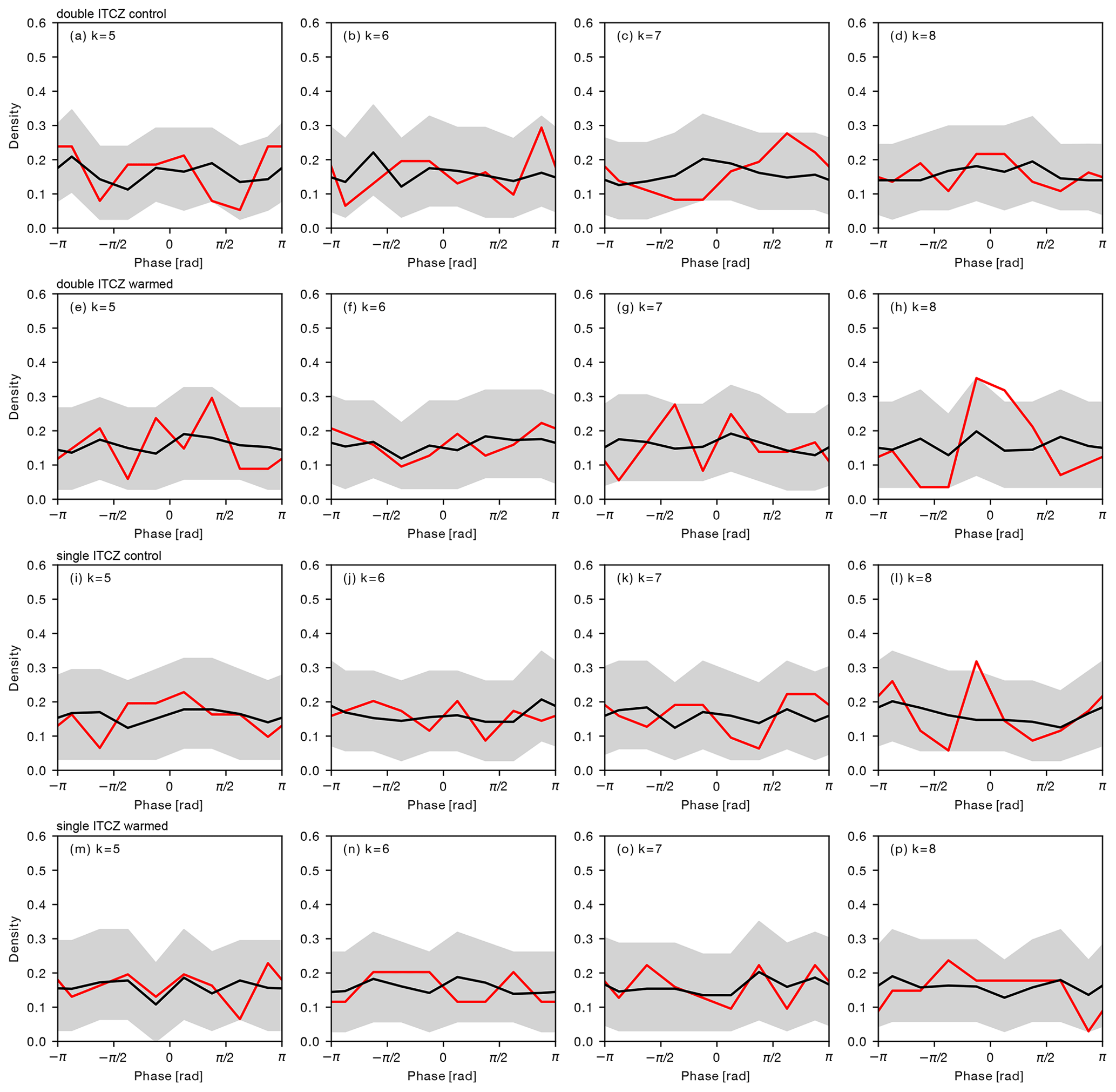
Figure 7Normalised histograms of phase positions for wavenumbers 5 (a, e, i, m), 6 (b, f, j, n), 7 (c, g, k, o) and 8 (d, h, l, p) for the double-ITCZ control simulation (first row), the double-ITCZ warming simulation (second row), the single-ITCZ control simulation (third row) and the single-ITCZ warming simulation (fourth row). The red line shows the histogram for the Nk high-amplitude weeks, and the grey shading and the black line show the 2.5 to 97.5 percentile range and the median for the randomly selected sets of weeks, respectively. The histograms were constructed using eight bins with width. The sample sizes Nk for individual panels range from 36 to 48 values.
Figure 7 shows histograms of the observed phase during weeks with high-amplitude waves for wavenumbers 5–8 (columns) and all four simulations (rows). As in Kornhuber et al. (2020), for some wavenumbers and simulations, there are rather large differences in the phase histograms for high-amplitude waves compared to climatology (compare red and black lines in Fig. 7), most notably for wavenumber 8 in the double-ITCZ warming and single-ITCZ control simulations. Nevertheless, the deviations between the histograms for high-amplitude weeks in almost all cases lie within the 2.5 to 97.5 percentile range of the bootstrapping samples. This range suggests that similarly large deviations can arise due to sampling uncertainty, i.e. because the sample of weeks with high-amplitude waves (36–48 values in this study, 44–47 values in Kornhuber et al. (2020)) is rather small. The few exceptions mentioned above (e.g. Fig 7h) should also be interpreted with care, as we perform multiple statistical hypothesis tests here (each at a significance level of 5 %), and thus some erroneous rejections of our null hypothesis (no preferred phasing) are expected.
That is to say, contrary to the large-get-stronger, small-get-weaker wave response discussed above, where a Rossby wave response to warming previously diagnosed in far more complex GCM simulations is indeed apparent in our APE simulations, we find no evidence for a preferred phasing of high-amplitude, quasistationary synoptic wavenumber waves in our simulations. This confirms our initial hypothesis and suggests that, similar to lower wavenumber quasistationary waves, a preferred phasing of high-amplitude synoptic waves in the real atmosphere is likely related to quasistationary forcing mechanisms and zonal asymmetries, such as topography and land–sea contrasts.
4.5 Changes in blocking
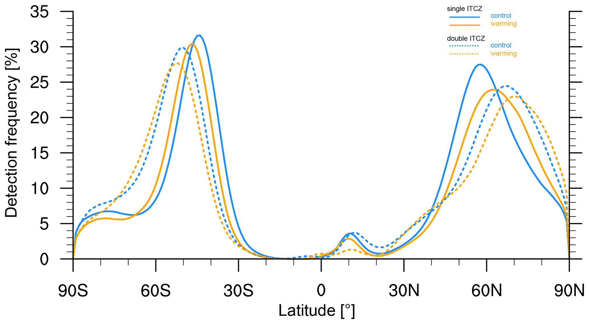
In the control simulation, zonal mean frequencies of blocking based on VAPV0 of approximately 4 % are found in the winter hemisphere's midlatitudes between 45∘ and 70∘ S (Fig. 8). The single-ITCZ simulation further features a pronounced and highly localised maximum in the subtropics, reaching frequencies of approximately 8 %. This maximum, which is not present in the simulation with a double ITCZ, coincides with the intense subtropical jet stream (Fig. 2b) and the associated steep climatological PV gradient (not shown). In the summer hemisphere, notable blocking frequencies are confined to poleward regions of 50∘ N with a maximum in both simulations located north of 60∘ N. In the double-ITCZ simulation, the maximum frequency is comparable in the winter and summer data, and the hemispheric average is considerably lower in summer due to the poleward shift in blocking occurrence. In the single-ITCZ simulation, the maximum frequency reaches only approximately half of that in the double-ITCZ simulation.
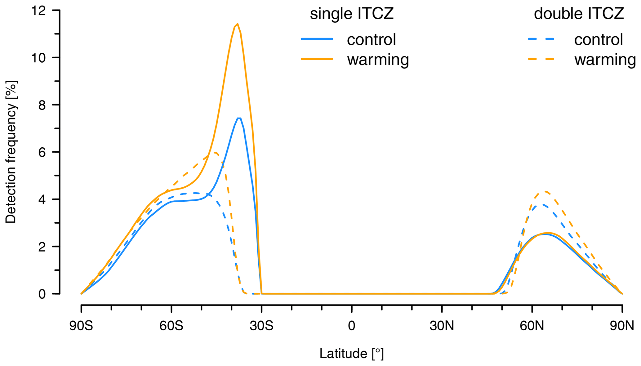
Figure 8Zonal mean detection frequency of blocks (see Sect. 2.4) weighted by cos(latitude) for control (blue; solid) and warmed (orange; solid) single-ITCZ and control (blue; dashed) and warmed (orange; dashed) double-ITCZ simulations. Blocking detection is based on VAPV0 and VAPVA for the control and warmed simulations, respectively.
As reported previously reported by Croci-Maspoli et al. (2007), changes in the tropopause height can potentially cause spurious trends in blocking frequency. In the warmed simulations, the tropopause is shifted upwards by 10–20 hPa (Fig. 5), which results in a reduction in the climatological VAPV0 compared to the control simulations (see circles in Fig. 9). Using VAPV0 for the identification of blocks in the warmed simulations results in a reduction in hemispheric blocking frequencies in summer, as well as in the case of the double-ITCZ simulation in winter. This change in blocking occurrence under warming is consistent with the spurious change expected due to a rise in the tropopause and an associated reduction in climatological VAPV0. To test for this possibility, we additionally performed the blocking identification in the warmed simulations with layers shifted upwards by 25 and 50 hPa, i.e. VAPV25 and VAPV50, respectively, thereby compensating for the effect of the elevated tropopause. Using VAPV25 or VAPV50 results in a positive change in climatological VAPV compared to the control, along with an increase in the hemispheric blocking frequency (plus and crosses Fig. 9) instead of a decrease. This points towards a high sensitivity of blocking detection to the choice of vertical layer and underlines that care must be exercised when comparing changes in blocking occurrence in such simulations of a warming climate.
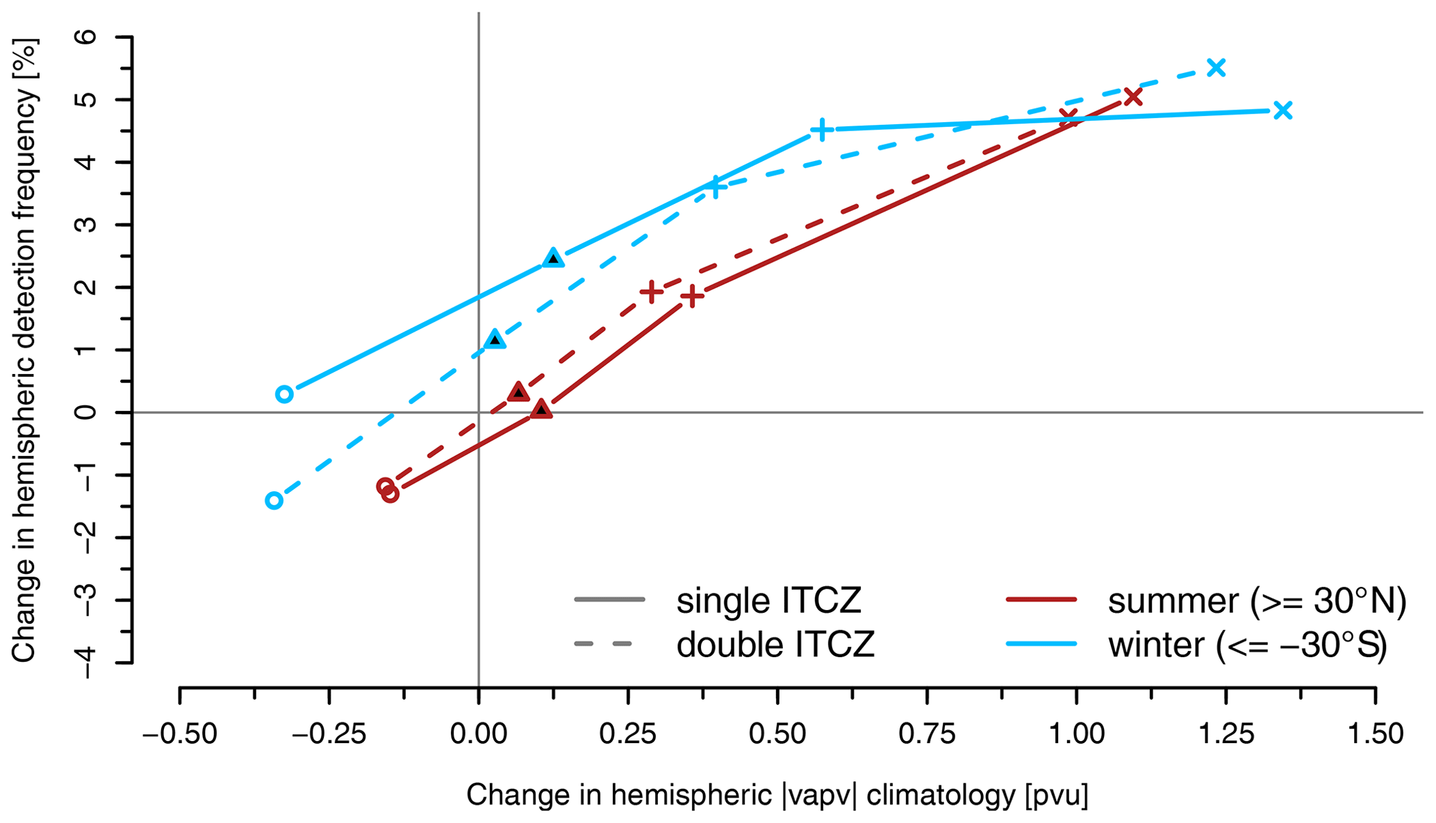
Figure 9Sensitivity of changes in blocking frequency to vertical shifts in the detection layer. The plot shows the change in hemispheric (poleward of 30∘ N or 30∘ S) VAPV climatology (x axis) and detection frequency of blocks (y axis) in warmed vs. control simulations with a single ITCZ (solid) and a double ITCZ (dashed). Red and blue indicate averages taken over the summer () and winter hemispheres (), respectively. Blocking detection in control simulations is based on VAPV0, whereas in warmed simulations, it is based on four different VAPV definitions: VAPV0 (circle), VAPV25 (plus), VAPV50 (cross) and VAPVA (black filled triangle).
We consider that VAPV as used for blocking identification should not change under warming. This is approximately true for VAPVA (black filled triangles in Fig. 9). In turn, we observe that under warming, zonal mean blocking frequencies remain nearly unchanged in the summer hemisphere, whereas they increase in the winter hemisphere (Fig. 8). The latter increase is largest in the subtropics in the single-ITCZ simulation and goes along with the intensification of the subtropical jet stream (Fig. 5b).
These sensitivities of the Schwierz et al. (2004) blocking identification scheme to a vertical expansion of the troposphere under warming are particularly relevant for interpreting previously reported blocking frequency trends derived from comprehensive GCM simulations. Several established blocking identification algorithms that have been used to this effect in previous studies (e.g. those featured in Woollings et al., 2018) work with pressure-level data. It is thus conceivable that negative trends in blocking frequencies identified in Woollings et al. (2018) are also affected by spurious effects due to the vertically expanding troposphere under climate warming.
4.6 Changes in surface cyclones
Feature-based detection of cyclones provides an opportunity to study the cumulative impact as well as the individual life cycle characteristics and changes in surface cyclones. In both simulations, the frequencies of cyclone detection are greater in the winter hemisphere (Fig. 10). Cyclone detection frequencies indicate the fraction of time steps a region is affected by a cyclone and range from 0 % (no cyclones) to 100 % (a cyclone is present at every time step) and the zonal mean is additionally scaled by the cosine of the latitude to account for the reduced circumference when going to the pole (the corresponding figure without scaling is shown in the Appendix). The largest frequencies in the zonal mean are found near 40–45∘ S in the single-ITCZ simulation (solid blue in Fig. 10). The storm tracks in the single-ITCZ simulation are, as expected, located closer to the Equator in both hemispheres than those in the double-ITCZ simulation. Consistent with the observations, the summertime storm tracks are located more poleward than the wintertime storm tracks.
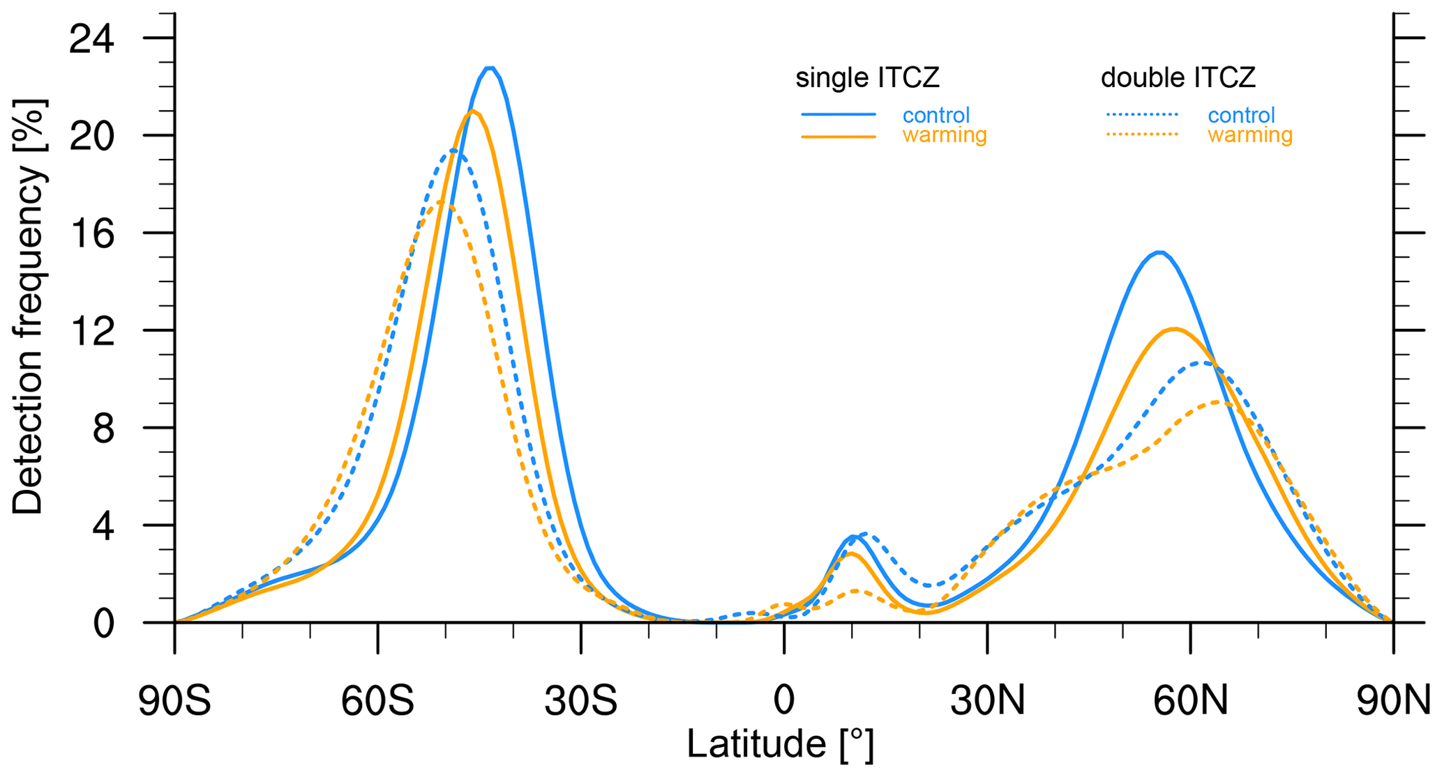
Figure 10Zonal mean cyclone frequencies weighted by cos(latitude) for (a) control (blue; solid) and warmed (orange; solid) single-ITCZ and (b) control (blue; dashed) and warmed (orange; dashed) double-ITCZ simulations.
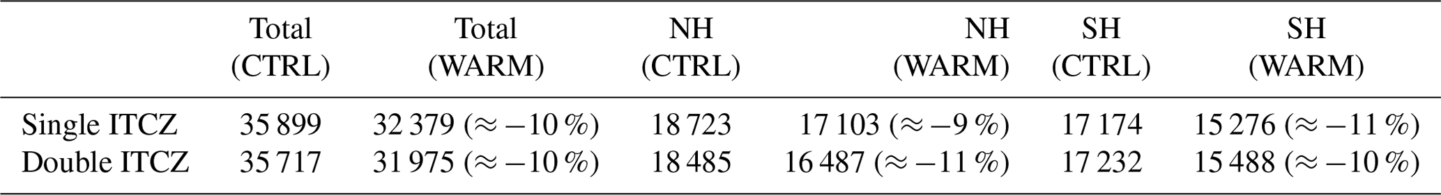
In the warmer simulations, peak cyclone frequencies decrease in both hemispheres and both simulation types. Several changes in life cycle characteristics can contribute to a change in the cyclone frequencies, for example a change in the number of cyclones (i.e. this tends to reduce the local cyclone frequencies) and their propagation speed (i.e. high propagation speed causes locally a reduced cyclone frequency) in combination with a reduction in their lifetime, which also tends to reduce the local detection frequencies. Table 1 summarises the number of identified surface cyclone tracks and their changes under warming. In agreement with previous studies (Sinclair et al., 2020; Schemm et al., 2022), the number of unique cyclones decreases in both simulations under warming. This reduction is of comparable order in the winter and summer hemispheres; for example, in the double-ITCZ run, the reduction in cyclone numbers is on the order of 10 %–11 %. It is also of similar order in the single-ITCZ run and in both hemispheres. Hence, cyclone numbers were reduced in general by approximately 10 % in this APE. Indeed, Zappa et al. (2013) and Chang et al. (2016) identify a reduction in the number of summertime extratropical cyclones in reanalysis data on the order of 4 % per decade over the entire Northern Hemisphere and regionally up to 10 %, for example over North America (Chang et al., 2016). The decrease in summertime extratropical cyclone activity is projected to continue into the future (Zappa et al., 2013; Chang et al., 2016).
Table 1Number of surface cyclone tracks and change relative to the control run in both simulation types and hemispheres (NH corresponds to the summer and SH to the winter hemisphere).
Changes in the lifetime of surface cyclone tracks are also considered. In agreement with a previous report (Schemm et al., 2022), the lifetime tends to decrease in both hemispheres. These changes are calculated based on a histogram of binned lifetimes, starting with lifetimes between 1 and 2 d and continuing in increments of 24 h to lifetimes of more than 2 weeks. The relative change values are then derived from the number of binned cases in the control and warmed simulations. The reduction is greatest for the long-lived cyclones in the summer hemisphere (Fig. 11a, b), but the large numbers also result from the small number of cases in the very long-lived cyclones. In the winter hemisphere (Fig. 11c, d), most lifetimes exhibit a similar decrease, except for the very long-lived cyclones, which indicate an increase. The results confirm the findings in Schemm et al. (2022), who identified an increase in lifetime, particularly for cyclones downstream of an additional SST front, which likely occurs due to an extension of the life cycle by diabatic processes. A drawback is the low numbers of long-lived cyclones and presumably the sensitivity of the result to cyclone identification and tracking. Hence, we consider the increase in long-lived cyclones to be less robust than the decrease in short-lived cyclones (up to 7000 cases in a hemisphere have a lifetime of 1–2 d compared to approximately 100 cases with a lifetime of more than 10 d).
This study introduces a simplified aquaplanet setup including winter and summer hemispheres to investigate the response of circulation to uniform warming in both hemispheres. Following the long tradition of previous aquaplanet experiments, a variant of the well-established zonally uniform “Qobs” SST distribution is introduced that allows us to mimic zonal mean June–July–August (JJA) SSTs as observed in reanalysis data. This SST distribution also allows us to control the formation of a double and single ITCZ, as observed over the East and West Pacific, respectively, depending on the cross-equatorial SST gradient. A 10-year simulation with radiation fixed at the equinox results in realistic large-scale circulation features, such as jet streams and storm tracks. The jet and the storm tracks are less intense and located more poleward in the summer hemisphere than in the winter hemisphere, which agrees with observations. The setup then is used to explore some challenging research questions related to changes in circulation with global warming, which we summarise below.
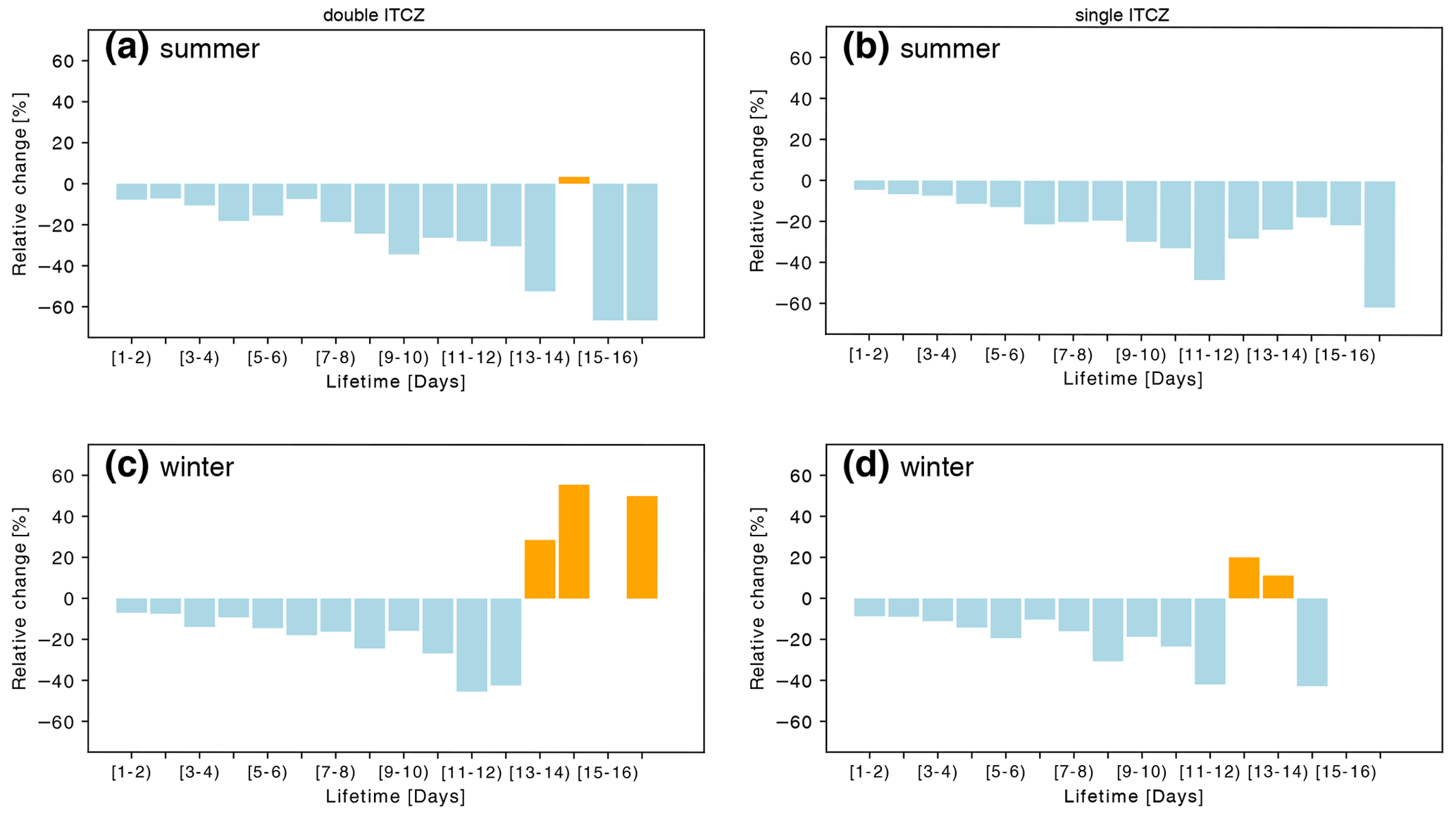
Figure 11Change in lifetime of surface cyclone tracks binned according to different lifetimes in days for (a, c) the double- and (b, d) single-ITCZ runs and for the summer (a, b) and (c, d) winter hemispheres.
Jet waviness. The waviness of the jet stream in a warmer climate has received much attention because of its association with extreme weather events (temperature and hydrological extremes) (e.g. Francis and Vavrus, 2015; Blackport and Screen, 2020). We choose a geometric definition of jet waviness based on isentropic 2 PVU contours (Röthlisberger et al., 2016). We first note that the waviness of isentropic 2 PVU contours increases climatologically when moving to lower isentropes. Therefore, if we examine the jet waviness at similarly valued isentropes (e.g. 320 K) in the control and warmed simulations, we find that the jet waviness increases. This spurious trend results from the fact that in the warmed simulation, the corresponding isentropes are closer to the surface. This trend is in agreement with arguments presented by Barnes (2013). Next, we compared the jet waviness on isentropes that are at the same height in pressure space identified from the zonal mean climatology. With this approach, we find that the jet waviness decreases. Finally, we compared the distribution of jet waviness when calculated at each time step on the isentrope with the highest wind speed (Martin, 2021). Again, the data show that the jet waviness decreases. There is only one exception to this decrease, which occurs at very high isentropes (e.g. 350 K) in the colder hemisphere, where the jet waviness increases and is not due to a change in the height of the isentrope. Overall, the observed upwards trend found by Martin (2021) is not reproduced in our zonally symmetric simulations of uniform warming, but based on our findings, a sensible way forwards is – as in Martin (2021) – to compare jet waviness on isentropes located at the jet maximum and not on isentropes or pressure surfaces held constant over time.
Rossby wave amplitude. A key result of our study is that our simulations, which feature no zonal asymmetries such as land–sea contrasts and topography, reproduce the large-get-stronger, small-get-weaker wave response to warming that was found by Chemke and Ming (2020) in fully coupled GCMs. The decrease in the amplitude of small waves (wavenumbers 7 and above) is greatest at jet stream levels and slightly equatorward of the mean jet position. This is consistent with the tendency of short waves to break cyclonically (Rivière, 2011). The increase in amplitude of large waves (wavenumbers 5 and smaller) is found mostly, but not exclusively, at lower stratospheric levels and within some distance of the jet stream. The increase tends to be stronger on the poleward side of the mean jet position, which agrees with the tendency of long waves to break anticyclonically (Rivière, 2011). The changes are found in both hemispheres, but they are more pronounced in the colder hemisphere. In the colder hemisphere, the increase in the amplitude of long waves at higher altitudes (i.e. 350 K) occurs near the location where we find an increase in the waviness of the jet. The reduction in jet waviness at lower isentropes (i.e. 320–330 K) and at the height of maximum wind speed is consistent with the reduction in synoptic wave amplitude, which dominates the change in wave amplitude at the jet core height. Note that the net waviness results from a combination of changes in all wavenumbers, but short waves contribute by a wider margin to the geometric jet waviness (i.e. due to more troughs and ridges and thus more latitudinal variations in the 2 PVU contour for short waves compared to long waves along a fixed-latitude circle). The increase in long-wave amplitude does not require zonal asymmetries as in the model of Moon et al. (2022), which neglects synoptic baroclinic wave growth, which in our case, however, dominates the wave amplitude changes at the height of the jet stream.
Rossby wave phase. During so-called high-amplitude wave events, Kornhuber et al. (2020) identified a preferred phasing of wavenumbers 5 and 7 in the Northern Hemisphere. While high-amplitude wave events are sometimes associated with concurring weather extreme events (Kornhuber et al., 2019; Rousi et al., 2022), the causes of this preferred phasing are currently unclear. As expected from the lack of topography and land–sea contrasts in our APE setup, we cannot identify a preferred phase of waves numbered 5–8 during weeks with anomalously large wave amplitudes, in neither the colder nor warmer hemisphere. We nevertheless explicitly present these results to motivate future studies on the causes of a preferred phasing of high-amplitude synoptic wavenumber waves based on our APE setup. In particular, we propose that our APE setup could be expanded, e.g. by adding idealised topography, SST fronts or comparable, to gain a mechanistic understanding of how this phenomenon comes about and to investigate to what extent forms of wave resonance might be involved (Charney and Eliassen, 1949; Petoukhov et al., 2016; Wirth, 2020; Wirth and Polster, 2021).
Blocks. Among all diagnostics used in this study, blocking detection based on PV vertically averaged between 500–100 hPa is the most sensitive to uniform warming and the associated rise in the tropopause. A spurious reduction in blocking frequencies results from the heightened tropopause in the warmer simulation (as already noted by Croci-Maspoli et al., 2007). A simple upwards adjustment of the VAPV in steps of 25 hPa, which accounts roughly for the tropopause lift, leads to an increase in detection frequencies but is also associated with an over-proportionally large increase in VAPV, potentially explaining the larger blocking frequencies. Once VAPV is very carefully tuned so that hemispheric-wide VAPV remains unchanged between the control and warmed simulations, blocking frequencies also remain unchanged in summer but still increase in winter. These results suggest that, rather than actual dynamical changes, the identified blocking frequency changes are predominantly a function of changes in the hemispheric VAPV in the vertical layer that is considered in the detection algorithm. Our confidence in the above-summarised blocking frequency changes thus remains low, even after the required adjustment. We therefore advise increased caution with trends derived from blocking detection schemes that are either directly or indirectly a function of pressure. Note that according to the review by Woollings et al. (2018), there is evidence of a reduction in blocking with global warming from a variety of detection algorithms and models. However, as some of these algorithms are pressure dependent, it is unclear to what extent this reduction is affected by vertical shifts in the tropopause, and it should be systematically investigated.
Surface cyclones. As noted in previous aquaplanet studies (Sinclair et al., 2020; Schemm et al., 2022), the number of cyclones decreases under warming. Here, it reduces globally by approximately 10 % and in the colder and warmer hemispheres. This reduction is already seen in reanalysis data; for example, Chang et al. (2016) find a reduction of up to 10 % over North America and of up to 4 % in the NH during summer since 1979 (until 2014). Zappa et al. (2013) report a projected reduction of 4 % (2 %) during NH winter (summer) over the North Atlantic under the RCP4.5 emission scenario, and this reduction is therefore a robust signal. Except for very long-lived cyclones in the colder hemisphere cyclone lifetimes decrease in both hemispheres.
Final remarks
Our study shows that feature-based detection methods need to be carefully adapted to new climates, in particular those that depend on a vertical coordinate. Moreover, it is shown that some circulation changes reported in the literature are already found in our zonally symmetric simulations under uniform warming, such as the change in wave amplitude of short and long waves, the stronger poleward shift in the storm tracks during summer compared to winter, and the dependence of jet waviness trends on the exact level and vertical coordinate. Other vividly discussed phenomena, however, are absent, such as the preferred phase of certain wavenumber waves during high-amplitude wave events.
In this study, we have argued and demonstrated that aquaplanet simulations such as those presented here may be useful tools for resolving questions regarding circulation changes in response to warming, predominantly for two reasons. First, they allow us to study the sensitivity of weather and circulation feature diagnostics to warming in a simplified setting, which helps unravelling and understanding which trends are methodological artefacts and which indeed relate to circulation changes. Second, they allow constraining the palette of causes of previously reported circulation changes and further allow highlighting or excluding the importance of changes in zonal asymmetries for these circulation changes. The data from our aquaplanet simulations are made publicly available (https://doi.org/10.3929/ethz-b-000644999), and it is hoped that they will serve as a starting point for subsequent studies on the debated topic of circulation changes under global warming.
Figure A1 shows normalised histograms of 6-hourly jet stream waviness for the winter hemisphere for (a) the 320 and 330 K isentropes in the control and warmed simulations, respectively. Panel (b) is similar but for the 330 and 340 K isentropes. Figure A2 shows normalised histograms of 6-hourly jet stream waviness on the isentrope with maximum zonal wind speed for the summer hemisphere in the simulation with (a) the double and (b) single ITCZ. The control is shown in blue and warmed in orange. At the point where the histogram appears cut off, the jet waviness is zero. The median and standard deviation shown on the bottom axis are based on the waviness distribution of the control run.
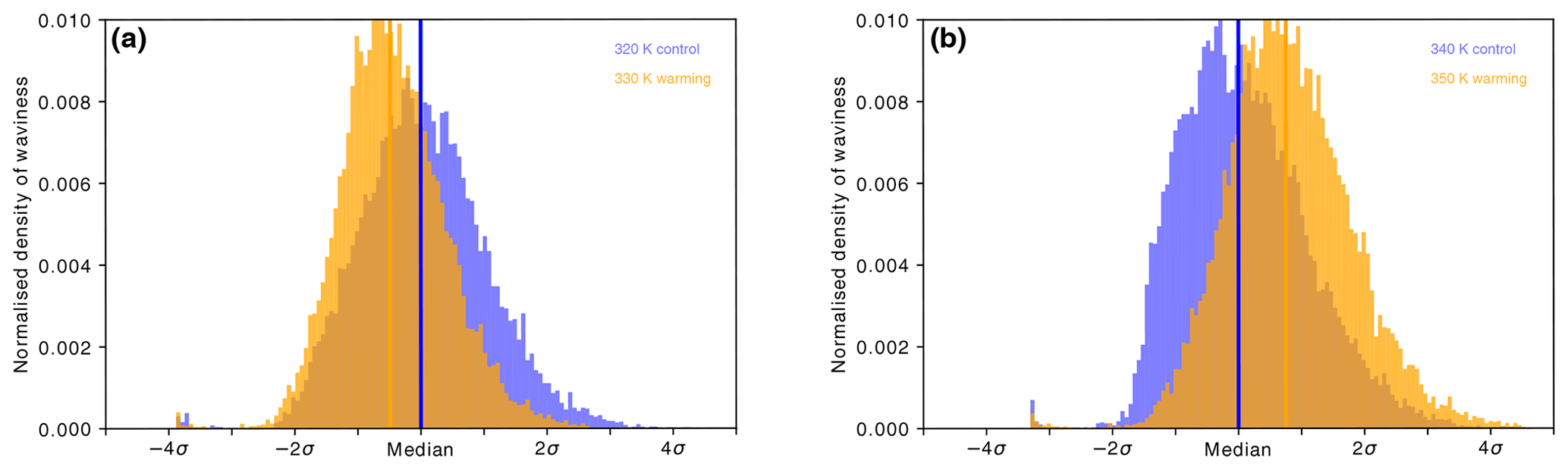
Figure A1Normalised histograms of 6-hourly jet stream waviness for the winter hemisphere for (a) the 320 and 330 K isentropes in the control and warmed simulations, respectively. Panel (b) is as (a) but for the 340 and 350 K isentropes.
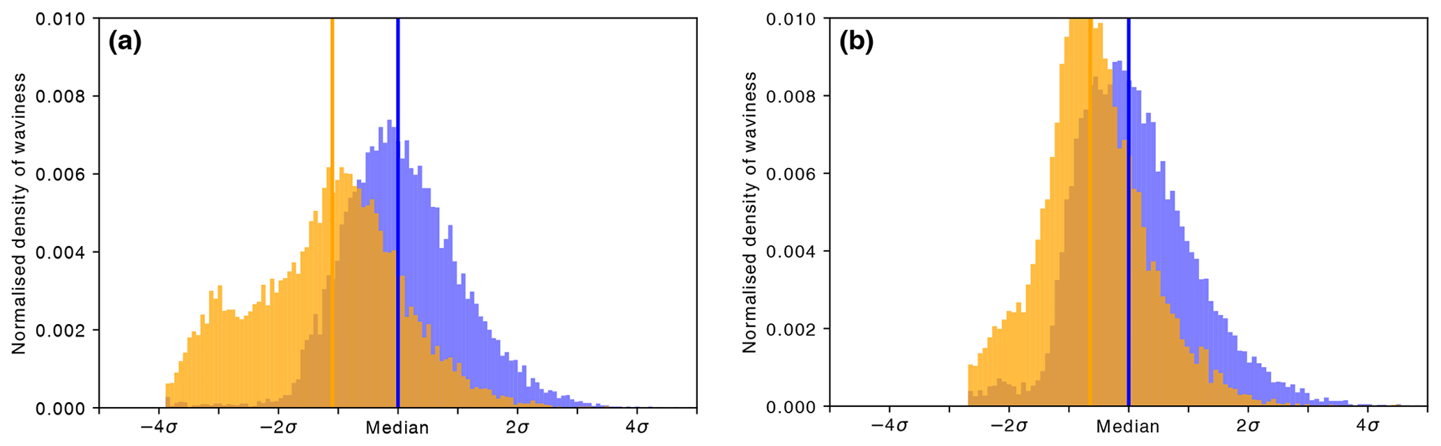
Figure A2Normalised histograms of 6-hourly jet stream waviness on the isentrope with maximum zonal wind speed for the summer hemisphere in simulations with (a) the double and (b) single ITCZ. Control is shown in blue and warmed in orange. At the point where the histogram appears cut off, the jet waviness is zero. The normalisation is done so that the integral over all bins is 1.
Zonal mean cyclone frequencies like in Fig. 10 but without cos(latitude) weight.
The ICON model is distributed to institutions under an institutional licence issued by the German Weather Service (DWD).
The primary data used for this paper are archived at ETH Zurich's Research Collection for scientific publications and research data under a CC-BY 4.0 licence for at least the upcoming 10 years (https://doi.org/10.3929/ethz-b-000644999, Schemm and Röthlisberger, 2023). ETH Zurich's Research Collection adheres to the FAIR principles.
SeS developed the APE setup and ran the simulations. MR led the analysis of the wave amplitude and the preferred phase position. SeS led the analyses of the waviness and the cyclone frequencies. SeS and MR led the writing of the manuscript.
At least one of the (co-)authors is a member of the editorial board of Weather and Climate Dynamics. The peer-review process was guided by an independent editor, and the authors also have no other competing interests to declare.
Publisher’s note: Copernicus Publications remains neutral with regard to jurisdictional claims made in the text, published maps, institutional affiliations, or any other geographical representation in this paper. While Copernicus Publications makes every effort to include appropriate place names, the final responsibility lies with the authors.
The authors acknowledge the work of Lukas Papritz, who investigated the required tuning of the block detection routine and performed the corresponding section. The Center for Climate Systems Modelling (C2SM) at ETH Zurich is acknowledged for providing technical and scientific support. All simulations were carried out at ETH's scientific and high-performance cluster EULER. Two anonymous reviewers are thanked for their constructive comments on the original manuscript.
Matthias Röthlisberger received funding from the INTEXseas project from the European Research Council (ERC) under the European Union's Horizon 2020 research and innovation programme (grant agreement no. 787652). Sebastian Schemm received funding from the GLAD project from a European Research Council (ERC) Starting Grant under the European Union's Horizon 2020 research and innovative programme (grant agreement no. 848698).
This paper was edited by Yen-Ting Hwang and reviewed by two anonymous referees.
Adam, O., Schneider, T., Brient, F., and Bischoff, T.: Relation of the double-ITCZ bias to the atmospheric energy budget in climate models, Geophys. Res. Lett., 43, 7670–7677, https://doi.org/10.1002/2016GL069465, 2016. a
Barnes, E. A.: Revisiting the evidence linking Arctic amplification to extreme weather in midlatitudes, Geophys. Res. Lett., 40, 4734–4739, https://doi.org/10.1002/grl.50880, 2013. a, b, c, d, e, f, g
Barnes, E. A. and Polvani, L.: Response of the midlatitude jets, and of their variability, to increased greenhouse gases in the CMIP5 models, J. Climate, 26, 7117–7135, https://doi.org/10.1175/JCLI-D-12-00536.1, 2013. a, b, c, d, e, f
Bischoff, T. and Schneider, T.: The equatorial energy balance, ITCZ position, and double-ITCZ bifurcations, J. Climate, 29, 2997–3013, https://doi.org/10.1175/JCLI-D-15-0328.1, 2016. a
Blackburn, M., Williamson, D. L., Nakajima, K., Ohfuchi, W., Takahashi, Y. O., Hayashi, Y.-Y., Nakamura, H., Ishiwatari, M., McGREGOR, J. L., Borth, H., Wirth, V., Frank, H. Bechtold, P. Wedi, N. P., Tomita, H., Satoh, M. Zhao, M., Held, I. M., Suarez, M. J., Lee, M., Watanabe, M., Kimoto, M., Liu, Y., Wang, Z., Molod, A., Rajendran, K., Kitoh, A., and Stratton, R.: The aqua-planet experiment (APE): CONTROL SST simulation, J. Meteorol. Soc. Jpn. Ser. II, 91A, 17–56, https://doi.org/10.2151/jmsj.2013-a02, 2013. a
Blackport, R. and Screen, J. A.: Insignificant effect of Arctic amplification on the amplitude of midlatitude atmospheric waves, Science Advances, 6, eaay2880, https://doi.org/10.1126/sciadv.aay2880, 2020. a, b
Brayshaw, D. J., Hoskins, B., and Blackburn, M.: The storm-track response to idealized SST perturbations in an aquaplanet GCM, J. Atmos. Sci., 65, 2842–2860, https://doi.org/10.1175/2008JAS2657.1, 2008. a
Brayshaw, D. J., Hoskins, B., and Blackburn, M.: The basic ingredients of the North Atlantic storm track. Part II: Sea surface temperatures, J. Atmos. Sci., 68, 1784–1805, https://doi.org/10.1175/2011JAS3674.1, 2011a. a, b
Brayshaw, D. J., Hoskins, B., and Blackburn, M.: The basic ingredients of the North Atlantic storm track. Part II: Sea surface temperatures, J. Atmos. Sci., 68, 1784–1805, https://doi.org/10.1175/2011jas3674.1, 2011b. a
Chang, E. K. M., Guo, Y., and Xia, X.: CMIP5 multimodel ensemble projection of storm track change under global warming, J. Geophys. Res.-Atmos., 117, D23118, https://doi.org/10.1029/2012JD018578, 2012. a
Chang, E. K. M., Ma, C.-G., Zheng, C., and Yau, A. M. W.: Observed and projected decrease in Northern Hemisphere extratropical cyclone activity in summer and its impacts on maximum temperature, Geophys. Res. Lett., 43, 2200–2208, https://doi.org/10.1002/2016gl068172, 2016. a, b, c, d, e
Charney, J. G. and Eliassen, A.: A numerical method for predicting the perturbations of the middle latitude westerlies, Tellus, 1, 38–54, https://doi.org/10.3402/tellusa.v1i2.8500, 1949. a, b
Chemke, R. and Ming, Y.: Large Atmospheric waves will get stronger, while small waves will get weaker by the end of the 21st Century, Geophys. Res. Lett., 47, e2020GL090441, https://doi.org/10.1029/2020gl090441, 2020. a, b, c, d, e, f, g, h
Chemke, R. and Polvani, L. M.: Linking midlatitudes eddy heat flux trends and polar amplification, npj Climate and Atmospheric Science, 3, 8, https://doi.org/10.1038/s41612-020-0111-7, 2020. a
Cohen, J., Zhang, X., Francis, J., Jung, T., Kwok, R., Overland, J., Ballinger, T. J., Bhatt, U. S., Chen, H. W., Coumou, D., Feldstein, S., Gu, H., Handorf, D., Henderson, G., Ionita, M., Kretschmer, M., Laliberte, F., Lee, S., Linderholm, H. W., Maslowski, W., Peings, Y., Pfeiffer, K., Rigor, I., Semmler, T., Stroeve, J., Taylor, P. C., Vavrus, S., Vihma, T., Wang, S., Wendisch, M., Wu, Y., and Yoon, J.: Divergent consensuses on Arctic amplification influence on midlatitude severe winter weather, Nat. Clim. Change, 10, 20–29, https://doi.org/10.1038/s41558-019-0662-y, 2019. a
Coumou, D., Lehmann, J., and Beckmann, J.: The weakening summer circulation in the Northern Hemisphere mid-latitudes, Science, 348, 324–327, https://doi.org/10.1126/science.1261768, 2015. a, b, c
Coumou, D., Di Capua, G., Vavrus, S., Wang, L., and Wang, S.: The influence of Arctic amplification on mid-latitude summer circulation, Nat. Commun., 9, 2959, https://doi.org/10.1038/s41467-018-05256-8, 2018. a
Croci-Maspoli, M., Schwierz, C., and Davies, H. C.: A multifaceted climatology of atmospheric blocking and its recent linear trend, J. Climate, 20, 633–649, https://doi.org/10.1175/JCLI4029.1, 2007. a, b, c, d, e
Doms, G., Förstner, J., Heise, E., Herzog, H.-J., Mironov, D., Raschendorfer, M., Reinhardt, T., Ritter, B., Schrodin, R., Schulz, J.-P., and Vogel, G.: A description of the nonhydrostatic regional COSMO model. Part II: Physical parameterization, Tech. rep., Deutscher Wetterdienst, Offenbach, Germany, http://www.cosmo-model.org/content/model/cosmo/coreDocumentation/cosmo_physics_4.20.pdf (last access: 12 January 2024), 2011. a, b
Fereday, D.: How persistent are North Atlantic–European sector weather regimes?, J. Climate, 30, 2381–2394, 2017. a
Francis, J. A.: Why are Arctic Linkages to extreme weather still up in the air?, B. Am. Meteorol. Soc., 98, 2551–2557, https://doi.org/10.1175/bams-d-17-0006.1, 2017. a
Francis, J. A. and Vavrus, S. J.: Evidence linking Arctic amplification to extreme weather in mid-latitudes, Geophys. Res. Lett., 39, L06801, https://doi.org/10.1029/2012GL051000, 2012. a, b
Francis, J. A. and Vavrus, S. J.: Evidence for a wavier jet stream in response to rapid Arctic warming, Environ. Res. Lett., 10, 014005, https://doi.org/10.1088/1748-9326/10/1/014005, 2015. a, b, c, d
Francis, J. A., Skific, N., and Vavrus, S. J.: North American weather regimes are becoming more persistent: Is Arctic Amplification a factor?, Geophys. Res. Lett., 45, 11414–11422, https://doi.org/10.1029/2018GL080252, 2018. a, b
Harvey, B., Cook, P., Shaffrey, L., and Schiemann, R.: The response of the Northern Hemisphere storm tracks and jet streams to climate change in the CMIP3, CMIP5, and CMIP6 climate models, J. Geophys. Res.-Atmos., 125, e2020JD032701, https://doi.org/10.1029/2020JD032701, 2020. a
Hassanzadeh, P., Kuang, Z., and Farrell, B. F.: Responses of midlatitude blocks and wave amplitude to changes in the meridional temperature gradient in an idealized dry GCM, Geophys. Res. Lett., 41, 5223–5232, https://doi.org/10.1002/2014gl060764, 2014. a
Hogand, R. J. and Bozzo, A.: A flexible and efficient radiation scheme for the ECMWF model, J. Adv. Model Earth Sy., 10, 1990–2008, 2018. a
Hoskins, B. and Woollings, T.: Persistent extratropical regimes and climate extremes, Current Climate Change Reports, 1, 115–124, 2015. a, b
Huguenin, M. F., Fischer, E. M., Kotlarski, S., Scherrer, S. C., Schwierz, C., and Knutti, R.: Lack of change in the projected frequency and persistence of atmospheric circulation types over Central Europe, Geophys. Res. Lett., 47, e2019GL086132, https://doi.org/10.1029/2019GL086132, 2020. a
Jablonowski, C. and Williamson, D. L.: A baroclinic instability test case for atmospheric model dynamical cores, Q. J. Roy. Meteor. Soc., 132, 2943–2975, 2006. a
Kornhuber, K., Osprey, S., Coumou, D., Petri, S., Petoukhov, V., Rahmstoorf, S., and Gray, L.: Extreme weather events in early summer 2018 connected by a recurrent hemispheric wave-7 pattern, Environ. Res. Lett., 14, 054002, https://doi.org/10.1088/1748-9326/ab13bf, 2019. a, b
Kornhuber, K., Coumou, D., Vogel, E., Lesk, C., Donges, J. F., Lehmann, J., and Horton, R. M.: Amplified Rossby waves enhance risk of concurrent heatwaves in major breadbasket regions, Nat. Clim. Change, 10, 48–53, https://doi.org/10.1038/s41558-019-0637-z, 2020. a, b, c, d, e, f, g, h, i, j
Kučerová, M., Beck, C., Philipp, A., and Huth, R.: Trends in frequency and persistence of atmospheric circulation types over Europe derived from a multitude of classifications, Int. J. Climatol., 37, 2502–2521, 2016. a
Kyselý, J. and Domonkos, P.: Recent increase in persistence of atmospheric circulation over Europe: Eomparison with long-term variations since 1881, Int. J. Climatol., 26, 461–483, 2006. a
Martin, J. E.: Recent trends in the waviness of the Northern Hemisphere wintertime polar and subtropical jets, J. Geophys. Res.-Atmos., 126, e2020JD033668, https://doi.org/10.1029/2020JD033668, 2021. a, b, c, d, e, f, g, h, i, j, k
Moon, W., Kim, B.-M., Yang, G.-H., and Wettlaufer, J. S.: Wavier jet streams driven by zonally asymmetric surface thermal forcing, P. Natl. Acad. Sci. USA, 119, e2200890119, https://doi.org/10.1073/pnas.2200890119, 2022. a, b, c, d, e
Nakajima, K., Yamada, Y., Takahashi, Y. O., Ishiwatari, M., Ohfuchi, W., and Hayashi, Y. Y.: The variety of forced atmospheric structure in response to tropical SST anomaly in the aqua-planet experiments, J. Meteorol. Soc. Jpn. Ser. II, 91A, 143–193, https://doi.org/10.2151/jmsj.2013-a05, 2013. a
Neale, R. B. and Hoskins, B.: A standard test for AGCMs including their physical parametrizations. II: Results for The Met Office Model, Atmos. Sci. Lett., 1, 108–114, https://doi.org/10.1006/asle.2000.0020, 2000. a, b
Neu, U., Akperov, M. G., Bellenbaum, N., Benestad, R., Blender, R., Caballero, R., Cocozza, A., Dacre, H. F., Feng, Y., Fraedrich, K., Grieger, J., Gulev, S., Hanley, J., Hewson, T., Inatsu, M., Keay, K., Kew, S. F., Kindem, I., Leckebusch, G. C., Liberato, M. L. R., Lionello, P., Mokhov, I. I., Pinto, J. G., Raible, C. C., Reale, M., Rudeva, I., Schuster, M., Simmonds, I., Sinclair, M., Sprenger, M., Tilinina, N. D., Trigo, I. F., Ulbrich, S., Ulbrich, U., Wang, X. L., and Wernli, H.: IMILAST: A community effort to intercompare extratropical cyclone detection and tracking algorithms, B. Am. Meteorol. Soc., 94, 529–547, https://doi.org/10.1175/BAMS-D-11-00154.1, 2013. a, b
Orr, A., Bechtold, P., Scinocca, J., Ern, M., and Janiskova, M.: Improved middle atmosphere climate and forecasts in the ECMWF model through a nonorographic gravity wave drag parameterization, J. Climate, 23, 5905–5926, https://doi.org/10.1175/2010JCLI3490.1, 2010. a
Petoukhov, V., Petri, S., Rahmstorf, S., Coumou, D., Kornhuber, K., and Schellnhuber, H. J.: Role of quasiresonant planetary wave dynamics in recent boreal spring-to-autumn extreme events, P. Natl. Acad. Sci. USA, 113, 6862–6867, https://doi.org/10.1073/pnas.1606300113, 2016. a, b, c, d
Priestley, M. D. K. and Catto, J. L.: Future changes in the extratropical storm tracks and cyclone intensity, wind speed, and structure, Weather Clim. Dynam., 3, 337–360, https://doi.org/10.5194/wcd-3-337-2022, 2022. a, b, c, d
Rivière, G.: A dynamical interpretation of the poleward shift of the jet streams in global warming scenarios, J. Atmos. Sci., 68, 1253–1272, https://doi.org/10.1175/2011jas3641.1, 2011. a, b, c, d, e, f, g, h
Roebber, P. J., Grise, K. M., and Gyakum, J. R.: The Histories of well-documented maritime cyclones as portrayed by an automated tracking method, Mon. Weather Rev., 151, 2905–2924, https://doi.org/10.1175/MWR-D-22-0287.1, 2023. a
Röthlisberger, M. and Martius, O.: Quantifying the local effect of Northern Hemisphere atmospheric blocks on the persistence of summer hot and dry Spells, Geophys. Res. Lett., 46, 10101–10111, https://doi.org/10.1029/2019GL083745, 2019. a
Röthlisberger, M., Pfahl, S., and Martius, O.: Regional-scale jet waviness modulates the occurrence of midlatitude weather extremes, Geophys. Res. Lett., 43, 10989–10997, 2016. a, b, c
Röthlisberger, M., Frossard, L., Bosart, L. F., Keyser, D., and Martius, O.: Recurrent synoptic-scale Rossby wave patterns and their effect on the persistence of cold and hot Spells, J. Climate, 32, 3207–3226, https://doi.org/10.1175/jcli-d-18-0664.1, 2019. a, b
Rousi, E., Kornhuber, K., Beobide-Arsuaga, G., Luo, F., and Coumou, D.: Accelerated western European heatwave trends linked to more-persistent double jets over Eurasia, Nat. Commun., 13, 3851, https://doi.org/10.1038/s41467-022-31432-y, 2022. a, b, c
Sampe, T., Nakamura, H., and Goto, A.: Potential influence of a midlatitude oceanic frontal zone on the annular variability in the extratropical atmosphere as revealed by aqua-planet experiments, J. Meteorol. Soc. Jpn. Ser. II, 91A, 243–267, 2013. a
Schär, C., Leuenberger, D., Fuhrer, O., Lüthi, D., and Girard, C.: A new terrain-following vertical coordinate formulation for atmospheric prediction models, Mon. Weather Rev., 130, 2459–2480, https://doi.org/10.1175/1520-0493(2002)130<2459:antfvc>2.0.co;2, 2002. a
Schemm, S. and Röthlisberger, M.: Primary data: Aquaplanet simulations with winter and summer hemispheres: The setup and circulation response to warming (ETH Research Collection, 2023), ETH Zürich [data set], https://doi.org/10.3929/ethz-b-000644999, 2023. a
Schemm, S., Papritz, L., and Rivière, G.: Storm track response to uniform global warming downstream of an idealized sea surface temperature front, Weather Clim. Dynam., 3, 601–623, https://doi.org/10.5194/wcd-3-601-2022, 2022. a, b, c, d, e, f, g, h
Schwierz, C., Croci-Maspoli, M., and Davies, H. C.: Perspicacious indicators of atmospheric blocking, Geophys. Res. Lett., 31, L06125, https://doi.org/10.1029/2003GL019341, 2004. a, b
Sinclair, V. A., Rantanen, M., Haapanala, P., Räisänen, J., and Järvinen, H.: The characteristics and structure of extra-tropical cyclones in a warmer climate, Weather Clim. Dynam., 1, 1–25, https://doi.org/10.5194/wcd-1-1-2020, 2020. a, b, c, d
Sprenger, M., Fragkoulidis, G., Binder, H., Croci-Maspoli, M., Graf, P., Grams, C. M., Knippertz, P., Madonna, E., Schemm, S., Škerlak, B., and Wernli, H.: Global climatologies of Eulerian and Lagrangian flow features based on ERA-Interim, B. Am. Meteorol. Soc., 98, 1739–1748, https://doi.org/10.1175/BAMS-D-15-00299.1, 2017. a, b
Tiedtke, M.: A comprehensive mass flux scheme for cumulus parameterization in large-scale models, Mon. Weather Rev., 117, 1779–1800, https://doi.org/10.1175/1520-0493(1989)117<1779:ACMFSF>2.0.CO;2, 1989. a
Walker, E., Mitchell, D., and Seviour, W.: The numerous approaches to tracking extratropical cyclones and the challenges they present, Weather, 75, 336–341, https://doi.org/10.1002/wea.3861, 2020. a
Wernli, H. and Schwierz, C.: Surface cyclones in the ERA-40 dataset (1958–2001). Part I: Novel identification method and global climatology, J. Atmos. Sci., 63, 2486–2507, https://doi.org/10.1175/JAS3766.1, 2006. a
Williamson, D. L., Blackburn, M., Nakajima, K., Ohfuchi, W., Takahashi, Y. O., Hayashi, Y.-Y., Nakamura, H., Ishiwatari, M., McGREGOR, J. L., Borth, H., Wirth. V., Frank, H., Bechtold, P. Wedi, N. P., Tomita, H., Satoh, M., Zhao, M., Held, I. M., Suarez, M. J., Lee, M., Watanabe, M., Kimoto, M., Liu, Y., Wang, Z., Molod, A., Rajendran, K., Kitoh, A., and Stratton, R.: The aqua-planet experiment (APE): Response to changed meridional SST profile, J. Meteorol. Soc. Jpn. Ser. II, 91A, 57–89, 2013. a
Wirth, V.: Waveguidability of idealized midlatitude jets and the limitations of ray tracing theory, Weather Clim. Dynam., 1, 111–125, https://doi.org/10.5194/wcd-1-111-2020, 2020. a, b, c
Wirth, V. and Polster, C.: The problem of diagnosing jet waveguidability in the presence of large-amplitude eddies, J. Atmos. Sci., 78, 3137–3151, https://doi.org/10.1175/jas-d-20-0292.1, 2021. a, b, c
Woollings, T., Gregory, J. M., Pinto, J. G., Reyers, M., and Brayshaw, D. J.: Response of the North Atlantic storm track to climate change shaped by ocean–atmosphere coupling, Nat. Geosci., 5, 313–317, 2012. a
Woollings, T., Barriopedro, D., Methven, J., Son, S.-W., Martius, O., Harvey, B., Sillmann, J., Lupo, A. R., and Seneviratne, S.: Blocking and its response to climate change, Current Climate Change Reports, 4, 287–300, https://doi.org/10.1007/s40641-018-0108-z, 2018. a, b, c, d, e, f
Zängl, G., Reinert, D., Rípodas, P., and Baldauf, M.: The ICON (ICOsahedral Non-hydrostatic) modelling framework of DWD and MPI-M: Description of the non-hydrostatic dynamical core, Quarterly Journal of the Royal Meteorological Society, 141, 563–579, https://doi.org/10.1002/qj.2378, 2014. a
Zappa, G., Shaffrey, L. C., Hodges, K. I., Sansom, P. G., and Stephenson, D. B.: A Multimodel assessment of future projections of North Atlantic and European extratropical cyclones in the CMIP5 climate models, J. Climate, 26, 5846–5862, https://doi.org/10.1175/jcli-d-12-00573.1, 2013. a, b, c, d
- Abstract
- Introduction
- Diagnostics
- An aquaplanet with a cold and a warm hemisphere
- Circulation response to uniform warming
- Conclusions
- Appendix A: Additional jet waviness histograms
- Appendix B: Additional zonal mean cyclone frequencies
- Code availability
- Data availability
- Author contributions
- Competing interests
- Disclaimer
- Acknowledgements
- Financial support
- Review statement
- References