A life cycle definition of year-round weather regimes in the North Atlantic European region

Weather regimes are quasi-stationary, persistent, and recurrent states of the large-scale extratropical circulation. Weather regimes explain most of the multi-day atmospheric variability on sub-seasonal time scales of 5 to 30 d. While regime definitions have been explored for the European region extensively, in recent years the existence of regimes in other world regions such as North and South America, and East Asia has been confirmed. Importantly, traditional regime definitions focus on a specific season and adapted approaches are needed for year-round applications. Using ERA-Interim reanalysis, Grams et al. (2017) introduced a year-round weather regime definition for the North Atlantic European region which accounts for inter-seasonal differences by construction. The study at hand now provides an update on ERA5 reanalysis data 1979–2019. It newly discusses commonalities, differences, and the rationale behind year-round North Atlantic European regimes compared to the canonical seasonal regimes, and presents a general overview of regime characteristics. The emphasis lays on inter-annual and intra-annual variability of regime occurrence. It is shown that the most extreme weather regime life cycles in terms of duration go along with extreme seasons in Europe, featuring heat waves, cold spells, or storm series. Finally, potential trends in regime occurrence are explored by extending the regime identification to the period 1950–2024. Overall inter-annual variability of regime occurrence dominates and there are hardly significant trends. Only Scandinavian Blocking shows a significant positive trend in summer and autumn in line with expected trends. The trend can be related to the thermal expansion of the troposphere under global warming but is highly sensitive to the methodology used. Next to present new insight in regime occurrence and trends, the paper aims to serve as a basis for subsequent work. It therefore also represents a thorough documentation of the seamless year-round definition of seven North Atlantic European weather regimes, and, accompanied with the open release of data and auxiliary scripts at Zenodo (Grams, 2025), it facilitates an easy start working with the year-round regimes.

1 Introduction

A large fraction of the variability of the large-scale extratropical circulation beyond the synoptic scale can be explained by a finite number of recurrent, quasi-stationary and persistent atmospheric states so-called weather regimes (Hannachi et al., 2017). Research on weather regimes has a long-standing history. Already early work by Namias (1950) pointed out that variability of extratropical weather is not only governed by baroclinic instability on synoptic scales of a few days and by seasonality, but also on what the scientific community today calls the sub-seasonal time scale (10–50 d). In particular, the phenomenon of “blocking” high pressure systems raised scientific attention. The fundamental study by Rex (1950a, b) established that these large-scale anticyclones can last for a few weeks, interrupt the usually prevailing westerly flow, and occur recurrently in similar locations. Subsequent work investigated weather regimes as metastable equilibrium states in the phase space of the atmosphere. This has been achieved by exploring solutions of non-linear statistical equations and dynamical system theory (Reinhold and Pierrehumbert, 1982; Vautard et al., 1988; Vautard and Legras, 1988; Palmer, 1993). In parallel, with the advent of larger gridded data sets of atmospheric (re-)analysis, typical weather regimes emerged from attempts to classify the large-scale circulation using pattern recognition (e.g. Barnston and Livezey, 1987; Kimoto and Ghil, 1993; Michelangeli et al., 1995). Together, this work established weather regimes as quasi-stationary, recurrent, and persistent states that explain variability of the large-scale extratropical circulation on time scales of about 10–50 d (Vautard, 1990; Michelangeli et al., 1995). Recent work by e.g. Michel and Rivière (2011), Faranda et al. (2016), Hochman et al. (2021), or Hauser et al. (2026) confirm that regimes are not a mere classification, but show a dynamical life cycle behaviour.

From a practical point of view, a key motivation for weather regimes lays in their link to surface weather. Weather regimes modulate weather conditions and the occurrence of extreme events on the large scale, e.g. aggregated over a country or continent-scale region, work pioneered by Yiou and Nogaj (2004). This raised particularly interest in the energy sector in the context of the renewable energy transition. It emerged that regimes modulate wind speed, and therefore wind power, on the critical multi-day time scale which is difficult to buffer in energy systems relying on a huge fraction of renewables (Santos-Alamillos et al., 2012; Santos et al., 2016; Zubiate et al., 2017; Grams et al., 2017). In Europe, periods of continent-wide lower than usual wind speed are of concern. It has been shown that this so-called “Dunkelflaute” is strongly linked to blocked regimes (Drücke et al., 2020; Mockert et al., 2023). The surface weather modulation by regimes also triggered applications in the health sector (White et al., 2021). Cassou et al. (2005) showed that increased heat-induced mortality in summer is linked to prolonged heat waves embedded in the European blocking regime. Similarly, Charlton-Perez et al. (2019) showed that cold-induced stress on the UK health system is linked to Greenland blocking.

Another practical application of regimes is sub-seasonal to seasonal (S2S) prediction. In the sub-seasonal forecast horizon, forecast skill is generally low and predictability emerges from slower varying modes of the Earth system, and thus, from boundary conditions rather than from initial conditions (White et al., 2017). It could be shown that the occurrence of European weather regimes is linked to such modes of variability. Cassou et al. (2005) showed that the occurrence of blocked regimes in summer is linked to anomalous tropical convection in the Caribbean and Sahel regions. Subsequent work unveiled the link of European weather regimes in winter to the Madden-Julian-Oscillation in the tropical Pacific (MJO; Cassou, 2008; Lin et al., 2009). Furthermore the occurrence of regimes in winter is modulated by the state of the stratospheric polar vortex with nuanced surface weather impact in Europe and North America (Charlton-Perez et al., 2018; Beerli and Grams, 2019; Lee et al., 2019b; Domeisen et al., 2020; Hauser et al., 2023a). Klaus (2017) and Lee et al. (2019a) showed that the MJO and stratospheric influence on regime occurrence in Europe is further modulated by ENSO. Notwithstanding the complicated details of these teleconnections, they provide a valuable source of S2S predictability for regimes and are seen as “windows of forecast opportunity” (Woolnough et al., 2024).

So far only few studies investigated how regimes change under global warming. A key problem is that climate models often show deficiencies in the representation of regimes in historic climate so that the interpretation of climate projections warrants caution. Notwithstanding, e.g. Santos et al. (2016) and Fischer et al. (2025) consistently report comparably small changes in regime frequency, but a more relevant change in surface weather through a likely thermodynamically-driven background signal. Fischer et al. (2025) argue, that despite the huge uncertainty in climate models the effect of frequency changes of regimes on changes in precipitation are likely smaller compared to the changes of precipitation associated with regimes themselves triggered by the thermodynamic effect of global warming. Although other studies stress changes in regime frequency and persistence in CMIP models (e.g. Fabiano et al., 2021; Dorrington et al., 2022b), it remains an open question if and how global warming already affects weather regimes and if this can be observed in circulation changes.

For the European domain, the 4 canonical winter regimes initially introduced by Vautard (1990) and Michelangeli et al. (1995) are widely used. In the last few years, weather regime definitions have also been established for East Asia (Matsueda and Kyouda, 2016) and North America (Lee et al., 2023). Still details of regime definitions, in particular the optimal number of regimes, how to treat seasonality, and how to optimize the explained variance, either in terms of large-scale flow variability or with a focus on surface impact, are topics of ongoing research: Different approaches have been used to investigate the variability in the large-scale extratropical circulation. The canonical European regimes emerge when analysing variables representative of the large-scale extratropical circulation such as mean sea level pressure or geopotential height. Intra-seasonal variability of the large-scale extratropical circulation has also been investigated in terms of different longitudinal positions of the eddy-driven jet (Woollings et al., 2010). Both perspectives can be reconciled as demonstrated by Madonna et al. (2017). Falkena et al. (2020) showed that an alternate approach in regime identification results in six instead of four regimes, which are more persistent while regime frequency does not alter. Most of the work on European weather regimes focussed on winter. However, as outlined in the Supplement of Cassou (2008) the regime patterns markedly differ in winter and summer.

Matsueda and Kyouda (2016) showed preferred winter circuits of regimes patterns for East Asian winter flow patterns, which enables the statistical prediction of a specific regime sequence. However, for the canonical European regimes it is difficult to identify such clearly preferred regime transitions. Previous studies emphasise the modulation of regime occurrence by external forcing such as tropical convection or the stratosphere (e.g. Cassou, 2008; Charlton-Perez et al., 2018; Beerli and Grams, 2019; Lee et al., 2019a; Domeisen et al., 2020; Mockert et al., 2025). Overall signals are relatively weak without considering a specific forcing, and the sample size is limited if forcing is accounted for (Klaus, 2017).

With a focus on applications in the energy sector Bloomfield et al. (2020) showed that targeted circulation types explain more surface weather-driven variance in renewable power output or electricity demand than weather regimes, but come with the caveat of being less related to dynamical regime behaviour. Weather regimes are not to be confused with weather types or the concept of “Grosswetterlagen”. Weather types, also called “weather patterns” (e.g. Neal et al., 2016), aim to explain synoptic day-to-day weather variability tailored to a specific region. Often 10–30 different weather pattern are distinguished. Weather regimes focus on a larger, continent-scale region and variability beyond the synoptic scale. For weather forecasting, a combination of weather patterns with a focus on day-to-day variability in the short- to medium-range forecast and on regimes beyond the medium-range turns out to be the most practical approach (Neal et al., 2016, 2024; Strommen et al., 2025). Similarly, Grams et al. (2020) stressed the need for regime definitions of different levels of complexity in order to balance the predictive signal and explained variance across lead times. Finally, Gerighausen et al. (2025) showed that a continuous description of regimes in addition to categorical regime thinking helps to tackle intra-regime weather variability.

For operational regime forecasts at ECMWF, Ferranti and Corti (2011) solved the problem of seasonally differing regimes, by gradual blending regimes centred on the current season throughout the year. So far these forecasts are the most common freely available operational product. Skill has been shown in both the medium-range (Ferranti et al., 2015) and sub-seasonal forecast horizon (Matsueda and Palmer, 2018), in particular in winter.

Grams et al. (2017) took a slightly different approach and introduced a year-round definition of seven North Atlantic European regimes complemented by a life cycle definition. These regimes distinguish three types of “cyclonic” regimes – Atlantic Trough (AT), Zonal regime (ZO), Scandinavian Trough (ScTr) – and four types of “blocked” regimes – Atlantic Ridge (AR), European Blocking (EuBL), Scandinavian Blocking (ScBL), and Greenland Blocking (GL). In addition it identifies roughly 30 % of all time steps as “no regime”. Their motivation was two-fold: From practical considerations in forecasting, seasonally changing regime patterns can cause confusion, as similarly named regimes go along with completely different flow patterns depending on the season. Second from a research-oriented perspective an objective life cycle definition enables studies on the dynamical behaviour and processes driving the occurrence of regimes. Expanding the number of regimes slightly, allows to better handle seasonality. Introducing a continuous regime index, in addition to a categorical regime attribution, allows better handling intra-regime weather variability.

Subsequently, the definition of seven year-round North Atlantic European regimes has been widely used in research and pre-operational forecast products have been developed together with ECMWF (Grams et al., 2020). The following gives an incomplete overview of the diversity of studies using these regimes. Several studies focussed on the modulation of extreme weather: E.g. Pasquier et al. (2019) showed how regimes modulate atmospheric river landfall in Europe, and thus, extreme precipitation. Papritz and Grams (2018) emphasised the role or regimes in cold air outbreaks over the Arctic Seas and the modulation of regime occurrence by the stratospheric polar vortex. Beerli and Grams (2019) showed the relevance of regimes for weather extremes relevant to the energy sector in winter, and their link to the state of the stratospheric polar vortex. Büeler et al. (2021) and Osman et al. (2023) documented forecast skill in S2S ensemble forecasts and worked out that European Blocking has least skill, stressing the importance to distinguish various types of blocking in the European region. Subsequently, Wandel et al. (2024) showed that it is the misrepresentation of the warm conveyor belt in these models which can explain the difficulties in predicting European blocking. The extensive study of blocked regime dynamics in Hauser et al. (2023b, 2024, 2026) sheds more light on the dynamical mechanisms during the onset of blocked regimes in the North Atlantic European region and emphasised the role of moist process upstream of the region where the regime establishes. This could only be achieved by focussing on objectively identified regime life cycle stages, e.g. regime onset. Focussing more on applications, Mockert et al. (2023) showed that cold Dunkelflauten in Germany are related to long-lasting Greenland blocking life cycles. Gerighausen et al. (2025) provides guidance for tackling intra-regime weather variability when using regimes for sub-seasonal prediction. Mockert et al. (2025) developed an ML-based postprocessing to improve sub-seasonal weather regime forecasts. Finally, the regimes raised also attention for impact research, e.g. in hydrological forecasting (Chang et al., 2023, 2025) and the investigation of compound extreme events (Brunner et al., 2025).

Despite the wide use, Grams et al. (2017) lacks a thorough documentation of the technical implementation as well as base characteristics of the year-round regimes. Such fundamental knowledge which would allow getting an overview about year-round regimes in the European region is so far scattered across a multitude of studies. Furthermore, regime data was only provided upon request, ERA-Interim is now outdated, and the regime attribution time series can no longer be extended. Also important technical details of the life cycle definition and recent changes coming with the update on ERA5 are hidden in the methodological description of subsequent studies, in particular Büeler et al. (2021) and Hauser et al. (2024).

The paper at hand aims to resolve these issues by providing an overview about the rationale behind the year-round North Atlantic European regimes, their characteristics, their use in previous studies and – for the first time – a discussion of potential trends in the occurrence of the seven year-round regimes. Thereby it also delivers the technical, conceptual, and scientific documentation of the year-round North Atlantic European regimes which is missing so far. Together with the public release of open data on Zenodo (Grams, 2025), this study establishes an easy starting point for future work.

The paper is structured as follows. Section 2 provides an overview of the data used. An overview of the technical implementation of year-round regimes is given in Sect. 3 together with details in Appendix A. Section 4 discusses the rationale behind the year-round life cycle definition, explains why seven regimes are optimal in the given configuration, how the seven regimes are related to each other and what are their commonalities and differences to the canonical seasonal four regimes. Section 5 provides a thorough discussion of key characteristics with a focus on their intra-annual, and inter-annual variability, extreme life cycles and surface weather. The potential implications of the effect of global warming on regime identification as well as potential trends are discussed in Sect. 6. The paper ends with a summary (Sect. 7) and concluding discussion (Sect. 8).

2 Data

This study is based on the global European Centre for Medium-Range Weather Forecasts (ECMWF) Re-Analysis 5 (ERA5; Hersbach et al., 2020). If not stated otherwise, data interpolated to a global grid at 0.5° horizontal grid spacing and with 3-hourly time steps from 1 January 1979, 00:00 UTC until 31 December 2019, 21:00 UTC is used. In addition, the backward extension (Soci et al., 2024) and near-real time continuation of ERA5 enables us exploring regime occurrence in the period 11 January 1950, 00:00 UTC until 30 June 2025, 21:00 UTC also on a global grid at 0.5° horizontal grid spacing and every 3 h. Analyses using this extended data period are indicated accordingly. The regime identification uses geopotential height at 500 hPa (Z500). Also the ERA5 surface variables mean sea level pressure (msl), 2 m temperature (2t), total precipitation (tp), 100 m wind components (100u, 100v), surface net short-wave radiation (ssr), and surface net short-wave radiation clear sky (ssrc)¹ are explored.

For radiation I compute the fraction of the daily accumulation of ssr and ssrc and refer to it as “solar insolation” (cf. Grams et al., 2017; Mockert et al., 2023). This quantity represents, on a given day, the fraction of the maximum possible daily insolation, accounting for seasonal differences in day length. I use solar insolation rather than total cloud cover due to its relevance to photovoltaic electricity generation.

In order to investigate the weather modulation during regimes, anomalies of surface weather variables are computed. The climatological reference period is 1979–2019. For 2 m temperature anomalies are calculated against a 30 d running mean climatology at the given hour. For total precipitation, 100 m wind speed (computed from the wind components), and solar insolation, anomalies are computed against a seasonal mean climatology. Seasons of interest are: winter (DJF – December, January, February), spring (MAM – March, April, May), summer (JJA – June, July, August), and autumn (SON – September, October, November).

3 Methodological summary and discussion of the Year-round regime definition

The year-round regime definition expands on established identification methods for the European domain, namely EOF analysis combined with clustering of Z500 anomalies (Michelangeli et al., 1995; Michel and Rivière, 2011; Ferranti et al., 2015). Key novel aspects are: (1) its seamless year-round implementation, achieved through a normalisation of Z500 anomalies with respect to the seasonal cycle in amplitude; (2) an objective identification of weather regime life cycles, the latter expanding on Michel and Rivière (2011); and (3) a categorical as well as a continuous regime classification for each time step. The regimes are defined using data in the 41 year period 1979–2019.

While this paper documents the intended application for seven year-round regimes in the North Atlantic European region, the implementation is flexible and can be applied to variables other than Z500, other world regions, and for reproducing the canonical seasonal regimes. The implementation has been tested for variables representing the large-scale flow (not shown); namely 200 hPa geopotential height (Z200) and upper-level (500–150 hPa) vertically averaged potential vorticity (following Schwierz et al., 2004), without finding added value compared to Z500 for regimes in the North Atlantic European region. Therefore, I stick to the established variable Z500. However, exploring Z200 enabled reproducing the seasonal North Pacific jet regimes of Winters et al. (2019), and using Z500 the East Asian weather regimes of Matsueda and Kyouda (2016) could be identified. Furthermore, Lee et al. (2023) followed the approach presented here to introduce year-round North American weather regimes. A further discussion of these excursions goes beyond the scope of this paper.

The remainder of this section outlines key steps and terminology used for the year-round regime definition. A comprehensive technical documentation, with the aim to ensure reproducibility is provided in Appendix A. The differences between regimes based on the initial version of Grams et al. (2017) using ERA-Interim and the current ERA5-based version introduced here are minor. These differences and the small technical adaptations in the regime definition are discussed in Appendix B.

3.1 Definition of the year-round regime patterns

In a first step seven year-round regime patterns are identified as follows. First, normalised 10 d low-pass filtered anomalies of Z500 (Z500^∗ in the following) are computed with respect to a 90 d running mean climatology (1979–2019). The normalisation removes the seasonal variability in amplitude while preserving spatial patterns. This ensures that regimes represent the variability in the large-scale flow pattern independent of the season. For technical details and a discussion of the effect of seasonality on regime identification I refer to Sect. A1 in the Appendix. Next an EOF analysis and fuzzy-c-means clustering are performed on 6-hourly Z500^∗ in the North Atlantic European domain 80° W to 40° E, 30 to 90° N and for the time period 11 January 1979, 00:00 UTC until 31 December 2019, 18:00 UTC (see Sect. A2). Seven clusters have been found to be optimal, as discussed in Sect. 4.1. I refer to these by the subscript wr with $\mathrm{wr}\in [\mathrm{AT},\mathrm{ZO},\mathrm{ScTr},\mathrm{AR},\mathrm{EuBL},\mathrm{ScBL},\mathrm{GL}]$ using the regime abbreviations introduced in the Introduction and explained in Sect. 4. Finally, the mean regime pattern in $\stackrel{\mathrm{‾}}{Z{\mathrm{500}}_{\mathrm{wr}}^{\ast }}$ according to the EOF-clustering is computed in geophysical space by averaging Z500^∗(t) of all 6-hourly time steps t attributed to a given cluster wr in the time period 11 January 1979, 00:00 UTC until 31 December 2019, 18:00 UTC.

3.2 Objective identification of weather regime life cycles and life cycle stages

The EOF-clustering categorises data according to some measure of similarity, and thus, is a mere statistical method without grounding in physics or dynamics. However, several studies pointed to a dynamic behaviour of weather regimes, and the existence of regime life cycles. A key novel step is the introduction of objective life cycles. These consider the gradual built-up of a regime as well as the gradual decay. The regime life cycles also account for the fact, that a regime onset might go on while the previous regime still decays (overlapping life cycles). The identification of regime life cycles is achieved by refining the use of weather regime indices I_wr introduced by Michel and Rivière (2011). I_wr are defined as the standardised projection of the instantaneous Z500^∗(t) on $\stackrel{\mathrm{‾}}{Z{\mathrm{500}}_{\mathrm{wr}}^{\ast }}$ and computed for each of the seven regimes. I_wr(t) is a simple scalar metric describing how well a regime wr is established at time t. Positive values indicate a positive correlation with the regime pattern, negative values an anti-correlation. One can see I_wr(t) also as a 7-dimensional vector encapsulating the current state of the atmosphere in the EOF domain in terms of Z500^∗, with the 7 scalar values describing how well each of the regime is established at a given time t. The latter thinking of I_wr(t) as a 7-dimensional vector has been used in, e.g., Mockert et al. (2025) for machine learning applications in S2S prediction and in Gerighausen et al. (2025) or Spaeth et al. (2024) for explaining intra-regime surface weather variability. Details on the computation of I_wr are given in Appendix A3.1.

Based on I_wr several objective regime life cycle stages are identified: the time of the onset (on), decay (dc), maximum projection (mx), as well as regime transitions (tr). The onset (on) describes the time step when a regime pattern is gradually building up and already established. Conversely, the decay (dc) describes the time step, when a regime pattern gradually dissolves and the regime pattern already vanished “to some degree”. This also implies that a regime life cycle might establish (or decay) while the life cycle of another regime is still active. Thus, it allows for overlapping life cycles, which makes sense from a dynamical perspective. The regime life cycles are identified in an iterative procedure by applying several criteria. Most importantly, the mean I_wr during a life cycle is larger than a given threshold thres_abs=1.0 and the life cycle must last for at least 5 d. Details and the rationale behind these criteria are given in Sect. A3.2 and Appendix A3.3.

In addition to the continuous description of regimes in terms of I_wr and overlapping life cycles, each time step is unambiguously attributed to a single regime simply by attributing it to the currently “dominant active regime”. This enables an additional categorical regime classification based on regime life cycles. The “dominant active regime” is the regime, which has an active life cycle at the given time and, if more than one active life cycle exists, the time step is attributed to the one with the maximum I_wr of all regimes with an active life cycle at that time. Intentionally, not all time steps belong to a regime life cycle following the attribution above, namely those for which no active life cycle exists. This filters out time steps when none of the regimes is well established (“no regime”). In fact, the defined threshold thres_abs=1.0 regulates to some degree how many time steps are not attributed to a regime. The threshold is chosen to allow approximately the same number of days attributed to a regime as the variance explained by the leading seven EOFs used for the EOF-clustering (see Appendix A2). The regime life cycle stages are best understood with an illustrative example which follows in Sect. 3.3. For trend analysis and climate monitoring Z500^∗, I_wr, and regime life cycles are extended to the period 11 January 1950, 00:00 UTC to 30 June 2025, 21:00 UTC in 3-hourly time steps, thus including the backward and forward extension of ERA5.

3.3 Illustrative example for weather regime life cycles

The episode of 20 February to 20 March 2018 serves as an illustrative example (Fig. 1). It was marked by a Greenland blocking (GL) which brought a cold surge towards Europe (cf. White et al., 2021; González-Alemán et al., 2022).

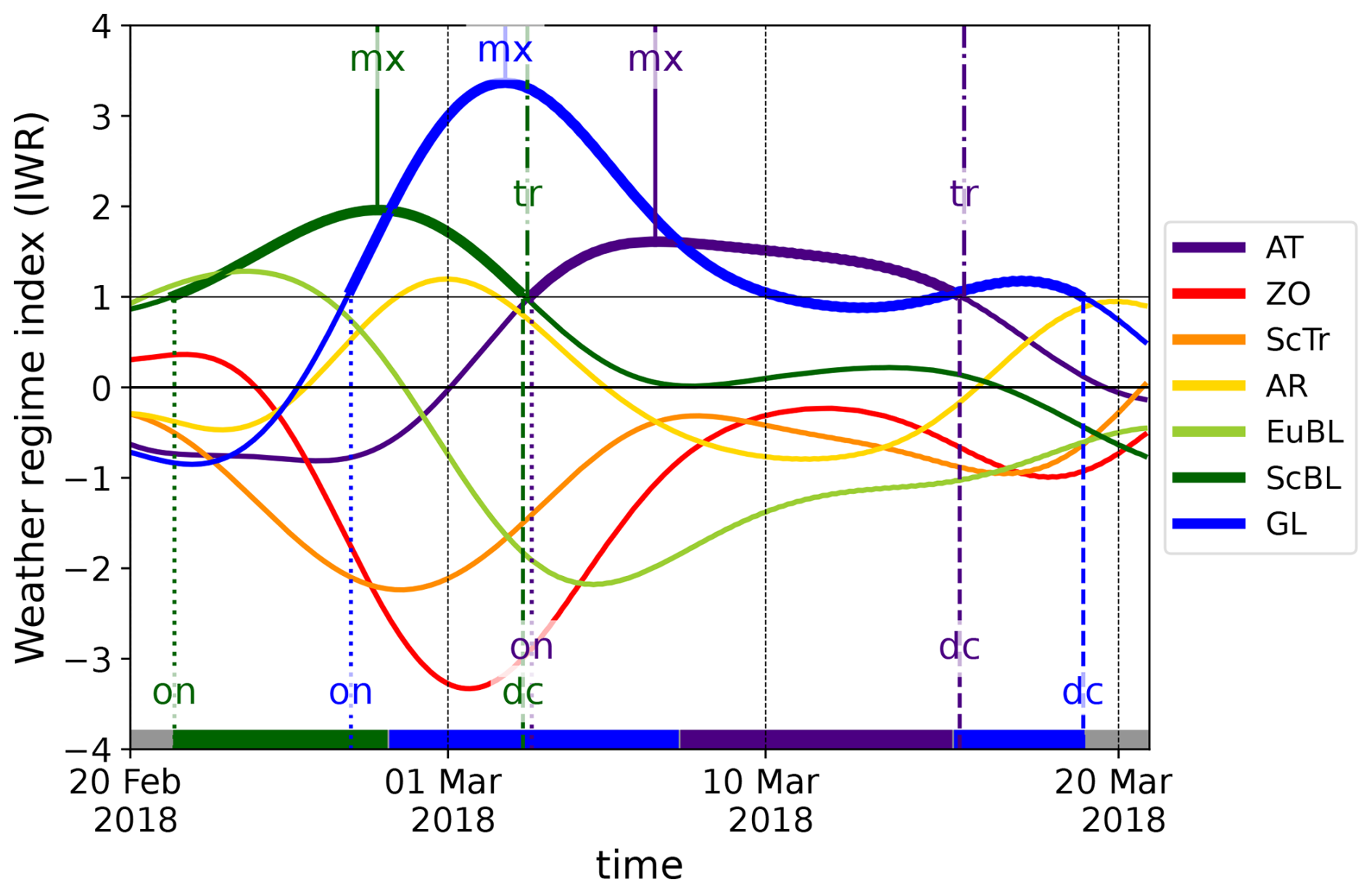
Figure 1 Time series of weather regime indices I_wr from 20 February 2018, 00:00 UTC until 20 March 2018, 21:00 UTC (coloured lines with wr according to legend). I_wr during active life cycles in bold. Thin dotted lines mark 1, 10, 20 March 2018, respectively. Coloured lines touching the respective I_wr curve mark life cycle stages: onset (on, dotted), maximum (mx, solid), decay (dc, dashed), and transitions (tr, dash-dotted). At the bottom of the figure the unambiguous categorical attribution of each time step to a regime is marked as coloured horizontal bar.

Looking at the categorical attribution of each time step (coloured horizontal bar at the bottom of Fig. 1 near y-axis value −4) shows that the episode begins with ScBL (dark green), followed immediately by GL (blue) until around 7 March. Then time steps are attributed to AT (violet) until 15 March, followed again by GL which decay in “no regime” (grey). This categorical view, reflects the “dominant active life cycle”, meaning the respective regime has a detected life cycle and its I_wr is the maximum of all I_w, w≠wr.

Much more information can be gained from the continuous I_wr time series. The period begins with a moderate projection onto weather regimes EuBL and ScBL (I_EuBL and I_ScBL around 1.0, green lines). On 21 February a ScBL life cycle begins with its maximum I_ScBL on 27 February. At that time a transition into a GL life cycle begins and the ScBL life cycle ultimately decays on 3 March (dark green). This is also when – out of the perspective of the ScBL life cycle – the transition tr to GL is objectively identified. The onset of that GL life cycle occurs on 26 February during the mature stage of ScBL. The GL life cycle reaches a very high I_GL of 3.4 on 2 March. During that time it has a “co-projection” into the decaying ScBL and AR (yellow), the latter not fulfilling the criteria of an own life cycle. The projection into ZO and ScTr are strongly negative, yet anti-correlated (in particular for ZO, which corresponds to the positive phase of the NAO, while GL corresponds to the negative phase). After the maximum stage a strong co-projection into AT (violet) occurs and a longer-lasting concomitant AT life cycle establishes from 3 until 15 March when it decays and transitions back into GL. The GL life cycle decays only on 19 March. During that long-lasting GL life cycle the AT life cycle is intermittently dominant from 7 to 15 March (violet).

This example served as illustration of regime life cycles and I am not not discussing the meteorological implications of the continuous I_wr and categorical perspectives for brevity. The interested reader is referred to the short discussion in Sect. 5.3, and the more in-depth discussions in Grams et al. (2020), and Gerighausen et al. (2025). The former stresses the utility of regime definitions of varying degree of complexity in forecasting. The latter highlights the importance of the continuous I_wr perspective for the interpretation of intra-regime surface weather variability.

4 Rationale behind a year-round weather regime life cycle definition

This section discusses why seven year-round regimes are a way to tackle caveats in regime definitions for Europe and how they differ and compare to the 4 canonical seasonal regimes. As discussed in the Introduction, the identification of weather regimes has a long-standing history, in particular in the North Atlantic European region. Thereby the methodological approach of using EOF analysis combined with clustering has been established as a standard procedure latest by Michelangeli et al. (1995). It has been subsequently used for the identification of the 4 canonical seasonal regimes which are consistent across studies and mostly identified for winter (e.g. Cassou, 2008; Ferranti and Corti, 2011; Michel and Rivière, 2011; Dawson et al., 2012; Ferranti et al., 2015). These 4 seasonal regimes are the positive and negative phases of the NAO (NAO+, NAO−; the latter also termed Greenland blocking), Atlantic Ridge (AR) and Blocking (BL; sometimes termed European Blocking or Scandinavian Blocking). However, it has been recognized that regimes substantially differ in winter and summer. Therefore separate seasonal identification has to be performed, yielding winter and summer regime “flavours”. For operational purposes Ferranti and Corti (2011) introduced a month-by-month adjustment of regime patterns to winter and summer patterns. Other studies preferred extended seasons. The Supplement of Cassou (2008) provides a comprehensive discussion of the problem and ambiguity of seasonality in regime identification. Still mostly the same names (NAO+, NAO−, BL, AR) are used for regimes in different seasons. From a user perspective this is confusing. Overall this motivated the year-round regime definition, aiming to represent both winter and summer regime “flavours” in one consistent framework. This has been achieved by the normalisations applied.

4.1 Finding an optimal number of year-round weather regimes

The optimal number of year-round weather regimes in the North Atlantic European domain has been determined by repeating the EOF-clustering while iteratively increasing the number of random seeds from k=2–11. An objective similarity index of the flow patterns in geophysical space, as well as expert judgement, independently determined k=7 as the optimal number of regimes. The stability of the clusters has been tested by repeating each configuration (k=2–11) ten times. These repetitions for fixed k always yield the same clusters. Thus, the clustering is insensitive to the choice of the random initial seeds. The similarity index is the maximum anomaly correlation coefficient (ACC_max) between the different clusters in a configuration with k prescribed clusters. The ACC is computed uncentred for the mean Z500^∗ field ($\stackrel{\mathrm{‾}}{Z{\mathrm{500}}_{\mathrm{wr}}^{\ast }}$, Sects. 3.1 and A2) for each pair and represents the pattern correlation between clusters (cf. Chap. 8.6.4 in Wilks, 2011). ACC scales between 1 and −1, meaning perfect correlation and anti-correlation, respectively. In forecast evaluation ACC above a threshold of 0.5 to 0.6 is considered as a reasonable good forecast (Wilks, 2011, and https://confluence.ecmwf.int/display/FUG/Section+6.2.2+Anomaly+Correlation+Coefficient, last access: 13 August 2025). Thus, computing the ACC between all clusters and retaining the maximum ACC_max gives an indication of how similar two clusters are within a given partitioning. As long as ACC_max remains below a certain threshold the clusters can be regarded as distinct.

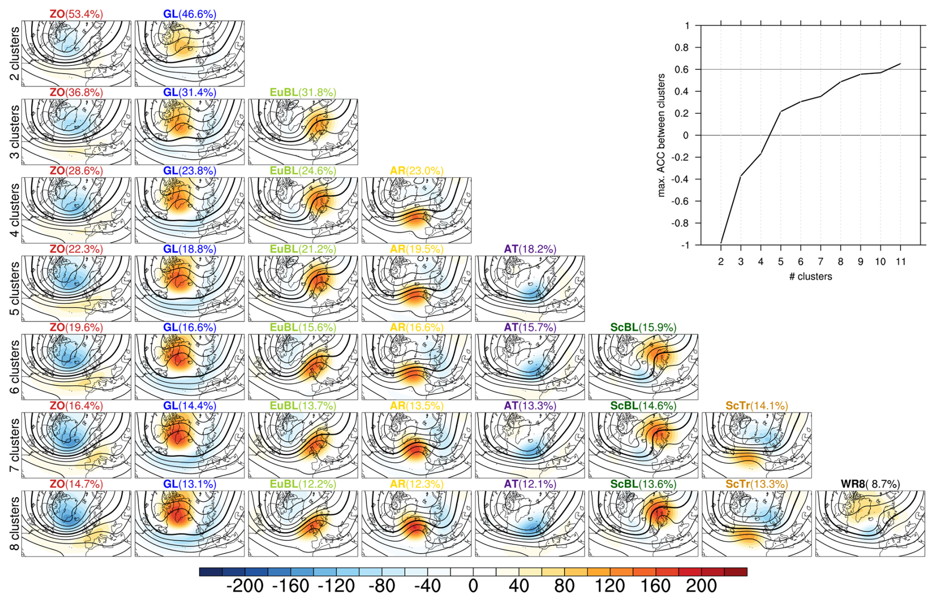
Figure 2 Comparison of different numbers of regimes (rows) for EOF-clustering of normalized 500 hPa geopotential height anomaly (Z500^∗). Denormalized fields of the cluster mean low-pass filtered Z500 anomaly ($\stackrel{\mathrm{‾}}{{\widehat{Z{\mathrm{500}}^{\prime }}}^{\mathrm{LF}}}$, shaded every 20 gpm) and absolute fields (contours every 80 gpm, 5520 gpm in bold) are shown. The panel labels indicate the regime name and the fraction of all dates 1979–2019 contained in the cluster. The inset in the top right corner indicates the ACC_max between different clusters (y-axis) for the configurations with increasing number of clusters selected a-priori for the clustering (x-axis).

Figure 2 shows the regime patterns based on the cluster mean of (non-normalised) 10 d low-pass filtered 500 hPa geopotential height anomalies ($\stackrel{\mathrm{‾}}{{\widehat{Z{\mathrm{500}}^{\prime }}}^{\mathrm{LF}}}$) with increasing number of clusters as well as ACC_max for k=2–11. With k=2 the patterns resemble the positive and negative phases of the NAO, here labelled “Zonal regime (ZO)” and “Greenland Blocking (GL)”, respectively. The two phases of the NAO are anti-correlated by definition. The method preserves this characteristic (see inset) despite using year-round data, the additional step of clustering, and reconversion in geophysical space. With increasing number of clusters, ACC_max rapidly increases but remains below 0 up to k=4 clusters. The k=4 clusters, although determined here from year-round data, still resemble the canonical seasonal regimes NAO+, NAO−, Blocking, and Atlantic Ridge. I am already using the corresponding labels ZO, GL, EuBL (for European blocking), and AR (for Atlantic Ridge). The amplitude of the Z500 anomalies are comparably weak, reaching locally below −120 gpm for ZO and above 140 gpm for AR.

With further increasing the number of clusters to k=5, 6, 7, more regime patterns emerge. These remain distinct to other patterns in the partitioning: ACC_max reaches only 0.35 for k=7. With k=5 the “Atlantic Trough (AT)” regime emerges with the negative geopotential height anomaly, and corresponding trough, shifted towards Europe compared to ZO. Distinguishing additional AT days makes also ZO, and GL somewhat sharper, reflected in an increase in mean amplitude of the anomalies and a signature of a ridge extending from the Azores to southwestern Europe emerging in ZO. With k=6 all the previous regime patterns remain, and “Blocking” splits up into EuBL (European Blocking) and ScBL (Scandinavian Blocking). As will become clear later, these are the winter and summer seasonal flavours of “Blocking (BL)” of the 4 canonical seasonal regimes, respectively. With k=7 all regime patterns sharpen further, while ACC_max hardly increases. The amplitude of $\stackrel{\mathrm{‾}}{{\widehat{Z{\mathrm{500}}^{\prime }}}^{\mathrm{LF}}}$ now ranges from −160 to 180 gpm. The additional “Scandinavian Trough (ScTr)” regime emerges. AR now has a pronounced positive anomaly up to 180 gpm in the Atlantic and a highly amplified Rossby wave pattern. At the same time ScTr is a variant with predominant negative anomaly and accompanying trough over Scandinavia while the ridge over the Atlantic remains comparably flat and the Rossby wave pattern is weakly amplified.

With k=8 the similarity between clusters jumps to a much higher level of 0.49, which is close to the threshold seen as a good forecast in forecast verification. Closer inspection of the regimes patterns reveals, that they hardly change neither in amplitude nor shape. Instead a relatively weak pattern “WR8” emerges which has a weak positive anomaly above 80 gpm stretching from the Nordic Seas to Greenland and a weak negative anomaly below −80 gpm south of Iceland. Thus, it resembles GL and somewhat AT and ScBL. In addition, much less days are contributing to WR8, compared to the other regimes. For k>8 clusters within a partitioning become even more similar. Because of the high values of ACC_max, thus high similarity, and the overall weak anomalies for k>7, k=7 has been found as the optimal number of regimes.

4.2 Description of the seven year-round regime patterns in terms of 500 hPa geopotential height

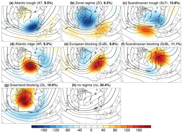
The set of seven year-round regimes provides a refined view on North Atlantic European weather regimes. Figure 3 shows the corresponding final large-scale flow patterns in terms of 500 hPa geopotential height, after applying the life cycle definition. Thus, in contrast to the raw EOF-clusters shown in the sixth row of Fig. 2, here “no regime” days are filtered out. This further sharpens the regime patterns: For the final year-round regimes ${\stackrel{\mathrm{‾}}{{\widehat{Z{\mathrm{500}}^{\prime }}}^{\mathrm{LF}}}}_{\mathrm{wr}}$ spans a range of about ±200 gpm (Fig. 3).

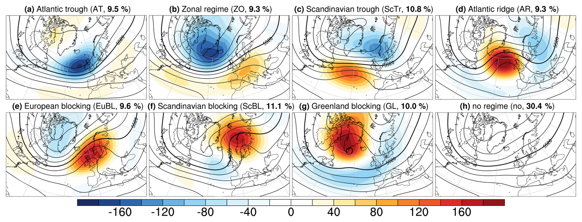
Figure 3 (a–g) Mean composites of 10 d low-pass filtered 500 hPa geopotential height anomalies (${\stackrel{\mathrm{‾}}{{\widehat{Z{\mathrm{500}}^{\prime }}}^{\mathrm{LF}}}}_{\mathrm{wr}}$, shaded every 20 gpm) and absolute field (black contours every 80 gpm, 5520 gpm in bold) for the seven year-round North Atlantic European weather regimes and “no regime” times (h). The composites are computed as the mean of ${\widehat{Z{\mathrm{500}}^{\prime }}}^{\mathrm{LF}}$ for all 3-hourly time steps 1979–2019 attributed to a regime wr according to the life cycle definition or “no regime” (see Sect. 3.2). Numbers in brackets indicate the annual frequency of the shown regime according to the life cycle attribution.

In a broad sense there are two groups of regimes. The “cyclonic regimes” AT, ZO, and ScTr compose the first group and are related to the positive phase of the NAO. They are dominated by a negative 500 hPa geopotential height anomaly and an accompanying large-scale trough (Fig. 3a–c). The cyclonic regimes also go along with enhanced cyclone activity, as reflected in the signature of mean sea level pressure and discussed in Sect. 5.4 (and cf. discussion of cyclone frequencies in Papritz and Grams, 2018). The “anticyclonic”, “blocked regimes” AR, EuBL, ScBL, and GL compose the second group. They are dominated by a positive Z500 anomaly. Again ZO and GL correspond to the positive and negative phases of the NAO, respectively. More details on the relationship of the seven regimes to the NAO index can be found in the Supplementary Table 1 in Grams et al. (2017) and, for winter, in Sect. 3.1 of Beerli and Grams (2019, their Fig. 2 and Table 1). Next, I briefly describe each of the seven regime patterns shown in Fig. 3.

ZO is characterised by a very strong and large negative geopotential height anomaly centred between Iceland and southern Greenland and a corresponding large-scale trough over that region (Fig. 3b). To the south a positive anomaly extends from the Azores into Europe with an accompanying flat ridge stretching from southwestern Europe to the Alps. Dense isohypses extend from North America to the North Sea, reflecting a well-established storm track (Fig. 3b). Importantly, the seven regimes distinguish the additional AT regime (Fig. 3a). The pattern of AT is shifted southeastward compared to ZO, with the negative anomaly centred west of Ireland. The region of the storm track is also shifted south and eastward with dense isohypses off the western European coasts. The ScTr regime features a negative geopotential height anomaly over the northern North Atlantic and Scandinavia accompanied by a flat ridge over the central North Atlantic and a corresponding positive Z500 anomaly (Fig. 3c). In summary, the mean 500 hPa geopotential height of the cyclonic regimes AT, ZO, and ScTr help distinguishing important variants of the positive phase of the NAO. These differences in regimes are important in terms of the surface weather modulation (Sect. 5.4).

The flat ridge accompanying ScTr (Fig. 3c) reminds of the canonical Atlantic Ridge regime in winter. In the seven regime definition AR exhibits a pronounced ridge over the North Atlantic embedded in an amplified Rossby wave pattern (Fig. 3d). The positive Z500 anomaly is located between the British Isles, Iceland, and southern Greenland, while a weaker negative anomaly prevails over Scandinavia and eastern Europe. Thus, the seven regime definition distinguishes well a cyclonic ScTr and an anticyclonic AR regime. A similarly better distinction of blocking situations over the European continent is evident for EuBL and ScBL. EuBL is characterised by a ridge over western Europe and a strong positive Z500 anomaly centred over the North Sea (Fig. 3e). The ridge axis is tilted anticyclonically. The patterns of ZO (Fig. 3b) and EuBL (Fig. 3e) both feature a dipole of Z500 anomalies: The negative anomaly over southern Greenland dominates in terms of amplitude in ZO, whereas the positive anomaly over Europe dominates in EuBL. In fact, on average EuBL projects in the positve phase of the NAO (see Supplementary Table 1 in Grams et al., 2017), underpinning the relationship between the cyclonic ZO and anticyclonic EuBL regimes. ScBL has a strong positive Z500 anomaly over Scandinavia with a highly amplified ridge tilted cyclonically towards Greenland (Fig. 3f). Upstream a marked trough off the Coast of western Europe goes along with a weak negative Z500 anomaly. As will be shown in the next section, EuBL and ScBL are the winter and summer variants of BL in the 4 canonical seasonal regimes, respectively. Furthermore, the 4 seasonal regimes would depict EuBL as AR in summer. Thus, the seven regimes allow a more refined view on blocking with the block either centred over the Atlantic (AR), western Europe and the North Sea (EuBL), or Scandinvia (ScBL).

Finally GL features a very strong and large positive geopotential height anomaly centred over southern Greenland and the Labrador Sea along with a very broad ridge in high latitudes (Fig. 3g). To the south a band of negative Z500 anomaly extends from North America into Europe. The accompanying zonally-oriented isohypses of Z500 reflect the southward shifted storm track during GL conditions. GL in some sense relates to the cyclonic AT regime. In contrast to GL, the negative Z500 anomaly dominates during AT situations, while a weak positive anomaly persists over the Baffin Bay. Finally, “no regime” days do not feature any discernible anomalies, thus Z500 is close to climatology (Fig. 3h). About 30 % of all days are attributed to “no regime”. The lack of anomalies indicates that these time steps constitute diverse large-scale flow situations which on average resemble the climatological mean.

With this description the “circle” of seven regimes closes. I have chosen the order of presentation (AT, ZO, ScTr, AR, EuBL, ScBL, GL) on purpose as it reflects the relationships between regimes. For completeness Fig. C2 shows the seasonally stratified field of 500 hPa geopotential height for all seven regimes. Note that the fields shown are non-normalised. Accordingly the maps primarily reflect the seasonal variation in the amplitude of geopotential height with winter featuring stronger gradients and anomalies compared to summer. By construction the overall regime pattern, independent of amplitude, are remarkable similar. This reflects the intent of the year-round definition focussing on the flow pattern rather than the amplitude.

4.3 Complementarity of the seven year-round regimes and the 4 canonical seasonal regimes

This section explains how the seven year-round regimes represent the 4 canonical seasonal regimes (cf. Michelangeli et al., 1995; Cassou, 2008; Ferranti et al., 2015). To this end, the regime framework has been applied to replicate the 4 seasonal regimes in DJF, MAM, JJA, and SON. This has been achieved by repeating the EOF-clustering for non-normalised 10 d low-pass filtered 500 hPa geopotential height anomalies (${\widehat{Z{\mathrm{500}}^{\prime }}}^{\mathrm{LF}}$; 1979–2019) in the respective season. Individual time steps are attributed to each regime according to the EOF-clustering. The life cycle definition has not been applied.

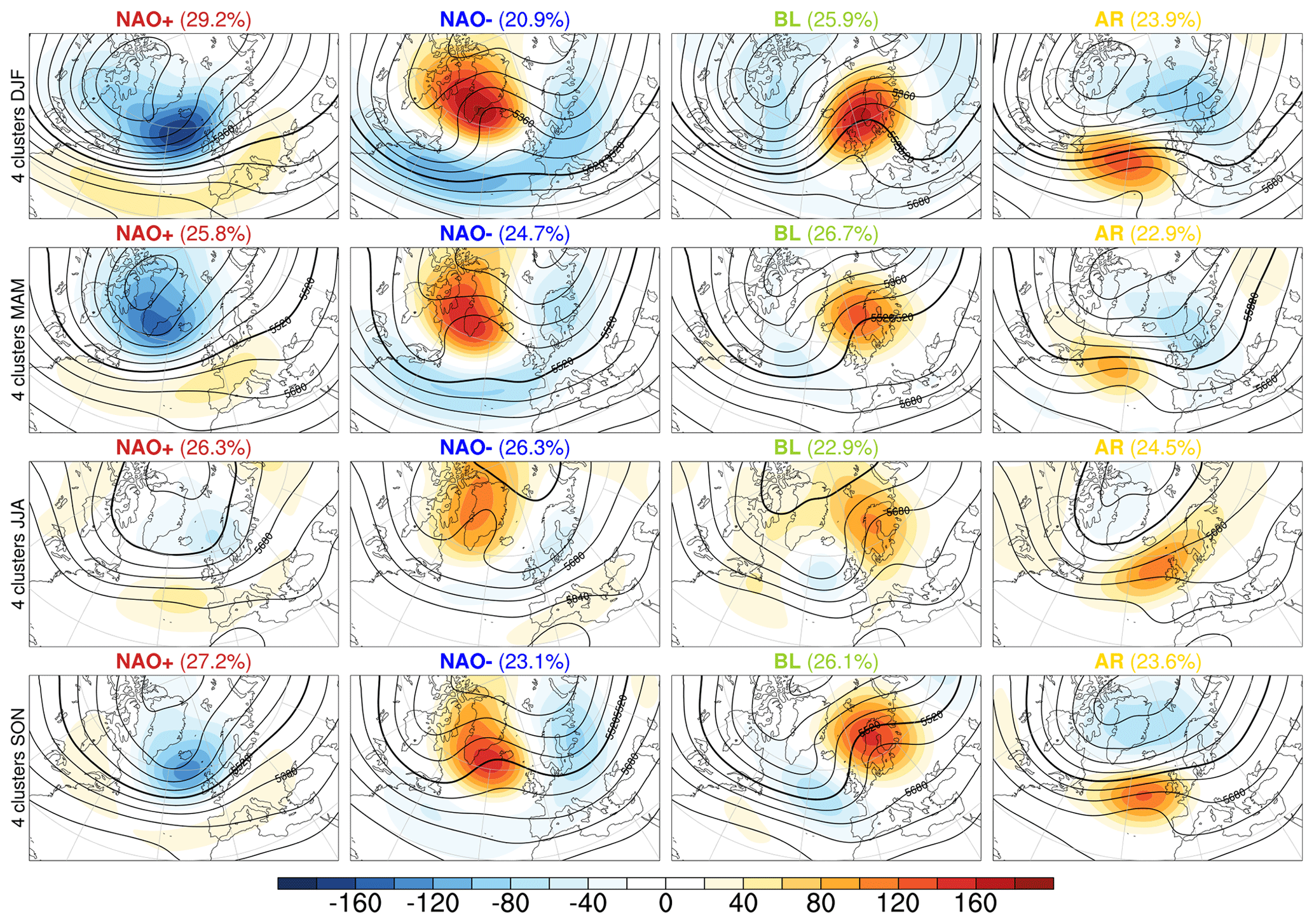
Figure 4 Mean composites of 10 d low-pass filtered 500 hPa geopotential height anomalies (${\stackrel{\mathrm{‾}}{{\widehat{Z{\mathrm{500}}^{\prime }}}^{\mathrm{LF}}}}_{\mathrm{wr}}$, shaded every 20 gpm) and absolute field (black contours every 80 gpm, 5520 gpm in bold) for variants with 4 seasonal North Atlantic European weather regimes and EOF-clustering applied to non-normalised 10 d low-pass filtered 500 hPa geopotential height anomalies (${\widehat{Z{\mathrm{500}}^{\prime }}}^{\mathrm{LF}}$) shown for each season. The composites are computed as the mean of ${\widehat{Z{\mathrm{500}}^{\prime }}}^{\mathrm{LF}}$ for all 6-hourly time steps 1979–2019 attributed to a regime wr according to their contribution to the EOF-clusters without applying the life cycle definition (see Sect. A2). Labels indicate the regime name abbreviation: NAO+ regime (NAO+), NAO− regime (NAO−), Blocking regime (BL), Atlantic Ridge regime (AR). Numbers in brackets indicate the seasonal frequency of the respective EOF cluster.

Figure 4 shows the 500 hPa geopotential height field calculated from averaging Z500 of all time steps contributing to the respective EOF cluster for the 4 canonical regimes in different seasons. In broad terms there is huge seasonal variability in the regime patterns and the amplitude of the Z500 anomalies. Seasonal regimes in winter (DJF) have much stronger Z500 anomalies of up to ±180gpm compared to summer (JJA, −60 to 100 gpm), the amplitude in transition seasons is in between. More importantly, the regime patterns change. For example, BL in winter has a pronounced ridge centred over western Europe, whereas in summer and autumn this shifts towards Scandinavia. Thus, in winter and summer BL resembles the EuBL and ScBL regimes of the year-round definition, respectively (cf. Fig. 3e, f). None of the seasonal AR variants (Fig. 4, right column) features a pronounced ridge over the Atlantic as it is the case for the seven year-round regimes (cf. Fig. 3d). Instead AR resembles ScTr in DJF and EuBL in JJA (cf. Fig. 3c, e). Also NAO+ (Fig. 4, left column) shows variants, which resemble more the three cyclonic regimes AT, ZO, ScTr depending on season (cf. Fig. 3a–c). These examples corroborate the introductory notion, of ambiguous regime naming, when using the same names for the 4 seasonal regimes in different seasons. These qualitative statements can be corroborated quantitatively, with an inspection of the attribution of all 6-hourly time steps 1979–2019 to either the 4 seasonal clusters or the seven regimes and “no regime” (Figs. 5 and C1).

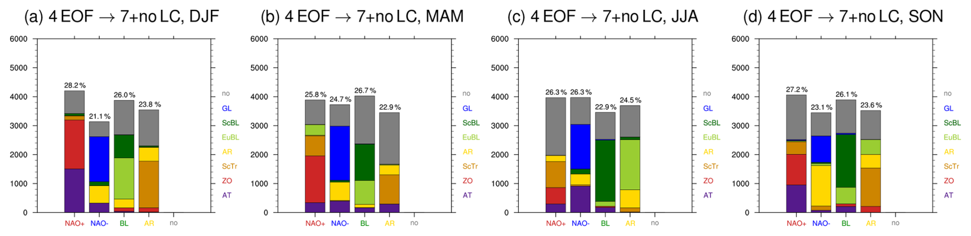
Figure 5 Frequency of the 4 North Atlantic European weather regimes according to the raw EOF-cluster attribution with 4 seasonal regimes defined for the seasons DJF (a), MAM (b), JJA (c), SON (d). Each bar show the number of 6-hourly time steps contributing to the seasonal regime with its name and colour code indicated on the x-axis and relative frequencies labelled. Coloured bar segments indicate how these time steps correspond to the 7+1 year-round regimes with labels and colour-coding for these to the right of each sub-figure. The inverse perspective of how the 7+1 regimes correspond to the 4 seasonal regimes is shown in Fig. C1.

All the seasonal variants of 4 regimes are well catered for by the 7 year-round regimes (Fig. 5). Most of the seasonal regimes correspond well to one of the seven year-round regimes, but with important seasonal differences. In winter (Fig. 5a), NAO+ corresponds to either AT or ZO of the seven regimes. NAO− is mostly covered by GL in all seasons. In winter AR of the 4 seasonal regimes is represented by ScTr of the seven regimes (Fig. 5a). The winter variant of BL of the 4 seasonal regimes is represented by EuBL of the seven regimes (Fig. 5a). Interestingly in summer (JJA; Fig. 5c) BL of the 4 seasonal regimes is represented by ScBL, as already qualitatively suspected above. In contrast now EuBL would represent the variant of AR of the 4 seasonal regimes. Thus, what would be seen as BL in winter and AR in summer using seasonal regimes, is in fact a similar pattern captured mostly by EuBL. This reflects the ambiguous name changes for regime patterns with seasons when applying a seasonal clustering. Also AT of the seven regimes helps to distinguish cyclonic situations from blocking, in particular in summer, when the 4 seasonal regimes classify AT situations as NAO− (Fig. 5c).

In summary, the seven year-round regimes well capture seasonal variants of regime behaviour. Key findings are: (1) A proper AR regime emerges, when ScTr and EuBL regimes help distinguishing the winter and summer contributions to the seasonal AR regime. (2) EuBL and ScBL are the winter and summer variants of the seasonal BL regime, respectively. (3) AT and ZO helps distinguishing important variants of NAO+. (4) GL or NAO− is relatively consistent across seasons.

5 Characteristics of year-round weather regimes in the North Atlantic European region

This section sheds more light on regime characteristics in terms of intra-annual and inter-annual variability of regime occurrence, duration of regime life cycles, preferred transitions, surface weather modulation, and extreme life cycles.

5.1 Intra-annual and inter-annual variability of regime occurrence

The year-round regime definition allows capturing distinct seasonal “flavours” of the canonical regime patterns as discussed before. This becomes apparent in the intra-annual climatology of regime occurrence (Fig. 6a). All seven regime and no regime happen year-round, however there are seasonal preferences: Atlantic trough (AT, violet) is the only regime which occurs with relative constant frequency year-round. The cyclonic Zonal (ZO, red) and Scandinavian Trough (ScTr, orange) regimes are more frequent in the winter half year (October to April) compared to summer (May to September). In particular ZO hardly occurs in peak summer (June to August). Also the occurrence of blocked regimes has some seasonality. Atlantic Ridge (AR, yellow) occurs relatively year-round with slightly enhanced frequency in autumn and winter (October to March). Likewise Greenland Blocking (GL, blue) occurs year-round with a preference for winter and spring (December to June), but reduced frequency in late summer and autumn (August to October). Most strikingly, the two types of blocking over the European continent, European Blocking (EuBL, light green) and Scandinavian Blocking (ScBL, dark green), have alternating seasonal preferences: While for both highest absolute frequencies occur in summer (June to September), the relative frequency between the two regimes alternates. In winter and spring (December to March), there is more EuBL compared to ScBL, while in summer (June to August), and to some degree in autumn (September to November), ScBL is the dominant type of blocking over the continent. “No regime” occurs year-round. Still spring is the season with the highest frequency of “no regime” days, likely reflecting the seasonal transition from storm track dynamics in winter, to less baroclinically driven weather systems in summer. This seasonal behaviour is also reflected when considering the cumulated frequencies of cyclonic (AT, ZO, ScTr; red shades together) vs. blocked regimes (AT, EuBL, ScBL, GL; yellow-green-blue shaded): cyclonic regime frequencies reach together up to 40 % in winter (December to February) but only 22 % in July. All blocked regimes together occur around 30 % of all winter days but more than 50 % in summer (June to August).

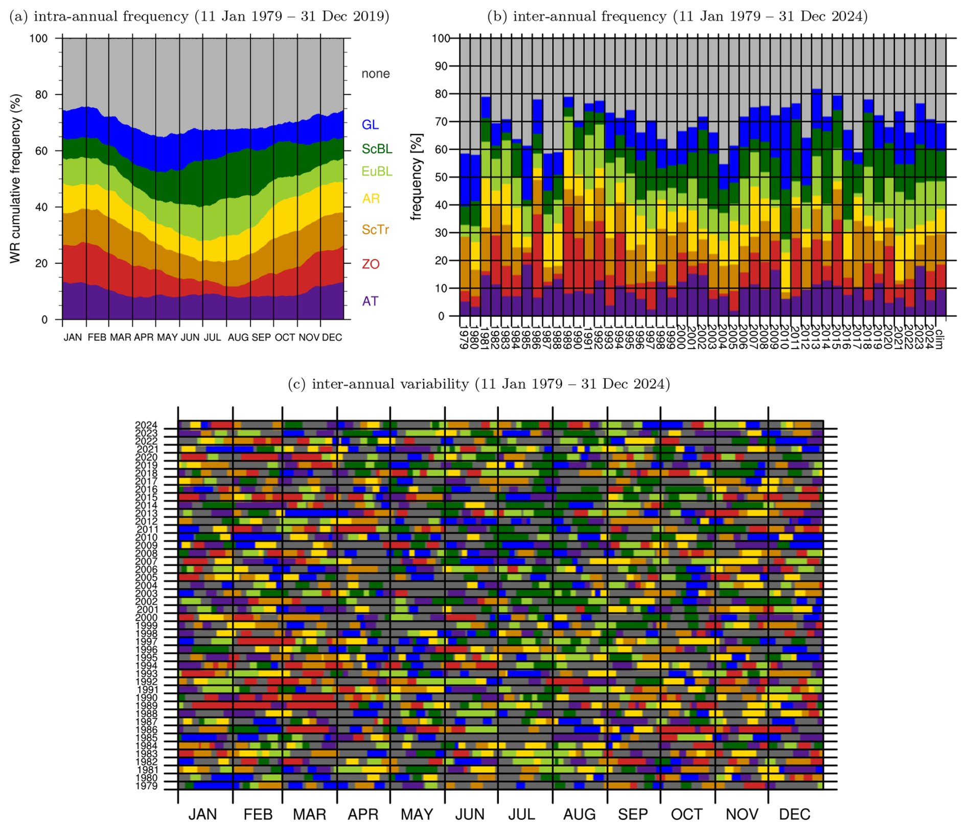
Figure 6 Intra-annual and inter-annual regime occurrence according to the unambiguous regime life cycle attribution of each calendar time (see methods). (a) Climatological mean regime frequency at each 3-hourly calendar time 1979–2019 smoothed with a 90 d running mean for each of the regimes. Colours represent each of the regime as indicated in the legend to the right. (b) Annual regime frequency in each year 1979–2024 (bars), and the climatological mean for comparison (right-most bar). (c) Similar to panel (b) but showing the life cycle attribution at each calendar time in the course of a year (horizontal dimension) to highlight intra-annual and inter-annual variability. Data period covers the period used for identifying regimes in panel (a), and the extension up to 2024 in panels (b) and (c).

The climatological mean frequency across the calendar year (Fig. 6a) helped to shed light on the seasonal variability of regime occurrence. A more refined view reveals important inter-annual variability in regime occurrence using the same data but stratified according to individual years (Fig. 6b). Hardly any of the individual years has the relatively even annual mean regime frequency of 9 %–11 % per regime. Instead, there are years which are particularly characterised by enhanced frequency of one or several regimes. For example, the early 1990s were characterised by a period of strong NAO+ conditions on seasonal to annual time scales, reflected in a very high frequency of the ZO and ScTr regimes in the years 1989–1994 and reduced occurrence of blocking. Vice-versa several individual years were characterised by enhanced blocking frequencies: 2010, with a dominant NAO− winter and consequently high frequency of GL, the very hot year 2003 in Europe with dominant occurrence of ScBL, or more recently the years 2021 and 2022 with frequent blocked regimes. A closer look to ScBL frequencies (dark green) in Fig. 6b gives the impression of an increase of the frequency in recent decades (also for EuBL, light green, and GL, blue, but weaker). Such potential trends are investigated in more detail in Sect. 6. For completeness Fig. C3 shows seasonal regime frequencies per year.

Combining the view on intra- and inter-annual variability in regime occurrence in one plot (Fig. 6c) confirms the huge inter-annual variability, but also the fact that cyclonic regimes occur more frequently in the winter half year (violet-red-orange shades) whereas blocked regimes occur more frequently in summer (blue and green shades). Subjectively it appears as if a recent increase in ScBL occurrence was driven by ScBL in summer and autumn. I will come back to a quantitative discussion of potential trends in regime occurrence in Sect. 6.

5.2 Regime duration and regime transitions

The period from regime onset until regime decay (see explanation of life cycle stages in Sect. A3.2) defines the life cycle duration. By construction of the definition of regimes used here, life cycles have a minimum duration of 5 d, which is reflected in the distribution of regime life cycle durations (Fig. 7a). The mean duration (dots in Fig. 7a) for all regimes is above 11 d (264 h) with life cycles of ZO reaching 13.5 d (300 h) on average. The median duration for all regimes is relatively equal ranging from 8.5 d (204 h) for EuBL up to 10 d (240 h) for ZO. Interestingly the cyclonic AT and ZO regimes tend to have the longest lasting regime life cycles, whereas blocked regimes tend to have shorter life cycles also with less variability in duration amongst the individual life cycles. EuBL is an exception with large variability of duration and the 75 % percentile reaching 15 d (360 h) as for ZO. The duration of regime life cycles somewhat depends upon the season (Fig. C4a–d). In particular GL life cycles are much longer in winter compared to summer with a mean duration of 15 d and the 25 % percentile above 11 d (blue in Fig. C4a). Compared to the duration of life cycles independent of the season (Fig. 7a) also EuBL in summer and ScBL and AR in autumn are much longer lasting (Fig. C4c, d). In conclusion, regime life cycles typically last for more than 10 d with some differences between different regimes and seasons. Recalling that the definition only prescribes a minimum temporal scale of 5 d (by low-pass filtering and the minimum duration criterion) this suggests a certain life cycle behaviour. Several studies confirmed that the regime definition applied here is not only a mere classification but identifies life cycles with a certain dynamical behaviour (e.g. Hochman et al., 2021; Hauser et al., 2024).

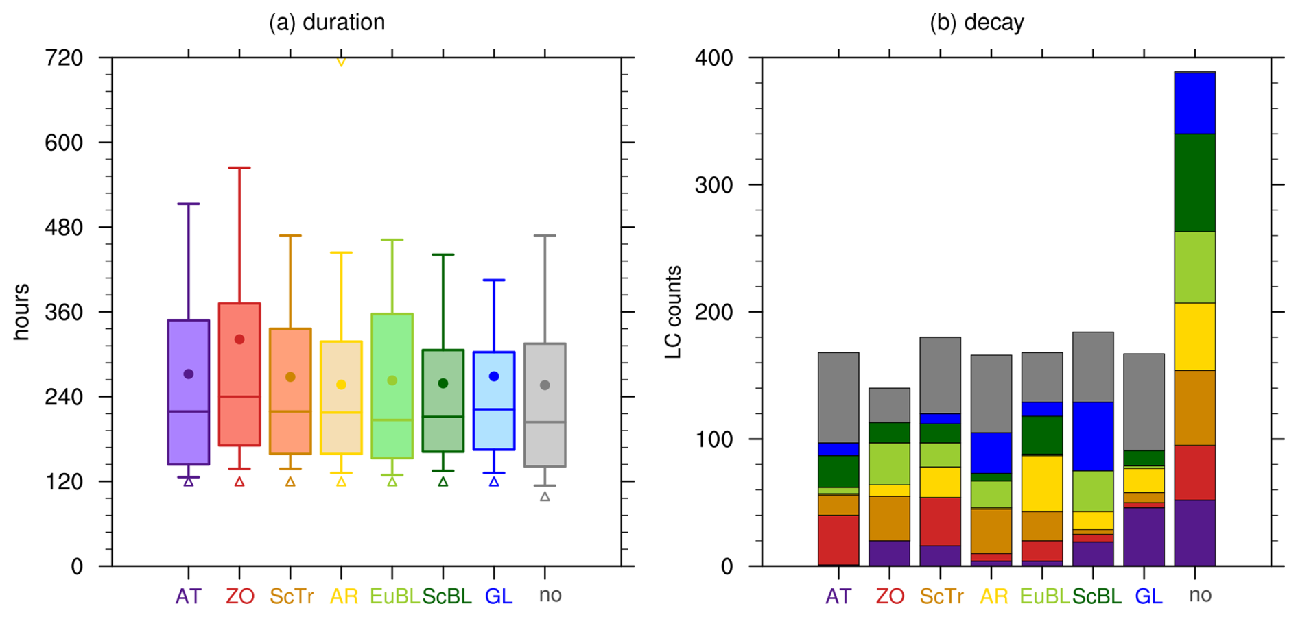
Figure 7 Duration and decay of weather regime life cycles. Box and whisker plots in panel (a) show distribution of duration from onset to decay for all regime life cycles of the respective regime (x-axis). Whiskers show the 10 % and 90 %, the box the 25 %, median, and 75 % percentile, respectively. Coloured dots show the mean and triangles the minimum duration. Bars in panel (b) show the number of life cycles (“LC counts”, y-axis) for each regime (x-axis) and the coloured segments in each bar the number of transitions into other regimes within a 4 d period after decay.

In contrast to East Asian regimes and similar to other definitions of European weather regimes (see discussion in Introduction), the seven year-round regimes show a huge variability of regime transitions (Fig. 7b) which primarily reflect the relationship between regimes (cf. Sect. 4.2). The next paragraph briefly discusses transitions defined as the presence of a new life cycle up to 4 d after a regime life cycle ended or following a “no regime” period.

First, a “no regime” period can be followed by any of the seven regimes, with a slight preference to ScBL in particular in summer and autumn (rightmost bar in Fig. 7b, Fig. C4g, h). The AT regime never transitions into AR, and most often ends in “no regime”, ZO, or ScBL. The ZO regime never transitions into GL, which echoes the opposite nature of the two phases of the NAO, represented by these two regimes. ZO has a somewhat higher tendency to transition into its related ScTr, EuBL and AT regimes. The ScTr regime can transition into any regime with the highest occurrence of a “no regime” period or a ZO or AR life cycle following ScTr decay. An AR regime can transition in any regime, but transitions into AT, ZO, and ScBL are rare. More likely are transitions into “no regime” and the related ScTr and GL regimes. Likewise EuBL preferentially transitions into the related AR or ScBL regimes or a “no regime” period. ScBL hardly ever transitions into ZO or ScTr, but most often into GL, and also into EuBL or “no regime”. The transition into GL reflects a preferred pathway of GL onset from a retrograding block over Scandinavia, revealed in the process-oriented study of Hauser et al. (2024). Finally GL most often transitions into “no regime” or AT. The latter reflects the relation of the NAO negative GL regime to the NAO positive AT, with both regimes featuring an equatorward shifted stormtrack but with altering dominance of either the block over Greenland or of the enhanced stormtrack (cf. discussion of GL and AT in Sect. 4.2). The overall picture of the transition behaviour holds also when stratifying according to season (Fig. C4e–h). The latter reflects more the seasonal preference of regime occurrence rather than fundamentally different transition behaviour in different seasons. In summary, regime transitions occur mostly into a “no regime” period or one of the related regimes. This behaviour is important for the impact of weather regimes in terms of surface weather modulation, as surface weather might change throughout a regime life cycle and in particular during transition periods (e.g. Beerli and Grams, 2019; Gerighausen et al., 2025).

5.3 Extreme regime life cycles

A natural question that might arise is about the characteristics of “extreme” regime life cycles. Different definitions of an extreme life cycle might be of interest, e.g., in terms of the life cycle duration, the mean I_wr, or the maximum I_wr. The Supplement provides tables with information about regime life cycles in the extended data period 1950–2024 ranked according to duration, mean I_wr, and maximum I_wr for a more in-depth analysis by interested readers. Here I briefly discuss some aspects of the regime life cycles with longest duration (Table 1). Relations to extreme events that affected Europe are mentioned inconclusively and informed by general knowledge and subjective verification in ERA5 analysis, using composites of 2 m temperature or 10 m wind speed anomalies against the data period 1990–2020 produced with Climate Reanalyzer (2025). These composites are provided as Fig. C5.

Table 1 Top 5 longest lasting regime life cycles in terms of duration. Columns contain the rank, the duration (in days), and the day of the begin of the life cycle (YYYYMMDD, where YYYY stands for the year, MM for month, DD for day of the onset time, the hour is omitted) for each regime, and rows stand for the rank 1–5.

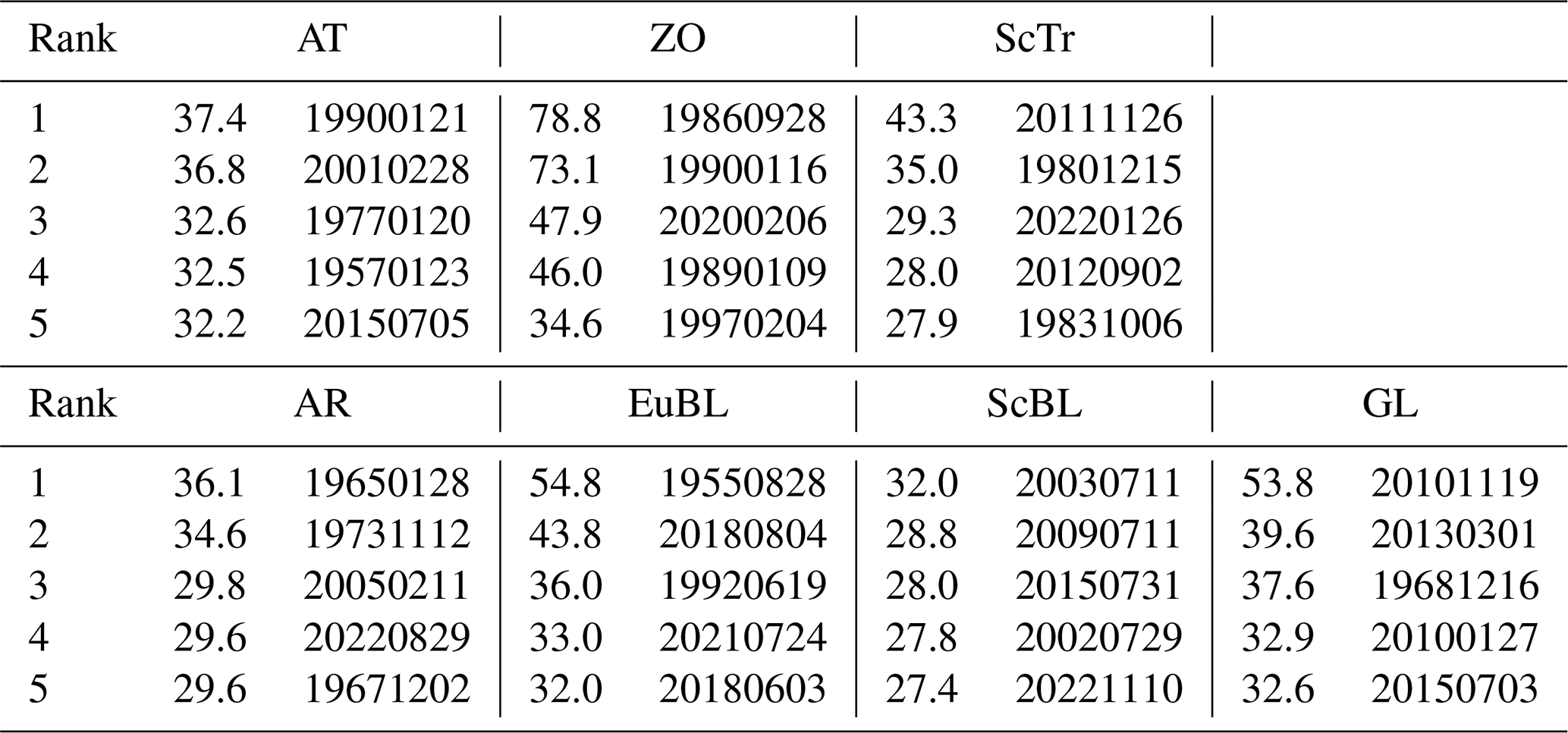
The longest lasting AT life cycle occurred in January and February 1990 and lasted for more than 37 d (Table 1). It overlapped with a ZO life cycle which lasted even for 73 d from January to March 1990. This was a period of severe winter storms in Europe (cf. Fig. C5b). Consistently, Hauser et al. (2023a) showed that serial cyclone clustering preferentially occurs in such well-established and long-lasting AT and ZO life cycles. The longest lasting life cycle of all regimes occurred in autumn 1986 for ZO and lasted almost 79 d, which was also a period with severe winter storms (cf. Fig. C5a). Consistent with the climatological occurrence preference of cyclonic regimes, the longest-lasting AT, ZO, ScTr life cycles almost entirely occurred in winter and autumn. An exception is AT, with the 5th longest life cycle in summer 2015, consistent with AT being the cyclonic regime which also has high occurrence frequency in summer and little seasonal preference.

Long-lasting blocked regime life cycles occur year-round (Table 1). However, it is remarkable that the longest ScBL life cycles entirely occurred in the 2000s and almost exclusively in summer, likely accompanied with heat waves. The longest lasting ScBL life cycle began in July 2003 and lasted 32 d, a summer during which Europe experience record-breaking heat (cf. Fig. C5c). Also the long-lasting EuBL life cycle in summer 2018 (44 d, rank 2) caused heat in Europe (cf. Fig. C5d). The longest-lasting GL life cycles preferentially occur in winter. The longest life cycle started in November 2010 and lasted for 54 d, followed by a 40 d lasting GL life cycle starting in March 2013. The latter was a response to a sudden stratospheric warming. Both long-lasting GL life cycles featured cold waves in Europe (cf. Fig. C5e, f), consistent with the finding of Mockert et al. (2023) that particularly long-lasting GL life cycles feature cold “Dunkelflauten”. The recent cold wave in March 2018 (cf. Fig. 1 and White et al., 2021) occurred during a GL life cycle ranked 5th in terms of maximum I_wr (not shown, see Supplement).

5.4 Modulation of surface weather

The modulation of surface weather on multi-day time scales and of the occurrence of extreme events is a key motivation for using weather regimes, in particular in sub-seasonal weather prediction.

Previous studies already extensively studied surface weather modulation during the seven year-round regimes. The following provides a brief overview of these studies. The original paper, Grams et al. (2017) (see also their Supplement), as well as Beerli and Grams (2019), Pickering et al. (2020) and Mockert et al. (2023) discuss surface weather modulation with relevance to renewable energies and a focus on wind, temperature, and insolation. Schaller et al. (2018) and Spensberger et al. (2020) focus on heat extremes, while Papritz and Grams (2018), Domeisen et al. (2020), White et al. (2021), González-Alemán et al. (2022), Mockert et al. (2023), Spaeth et al. (2024), and Kiefer et al. (2024) focus on cold extremes in Europe. The Bachelor thesis of Gerighausen (2022) studied the modulation of the likelihood of temperature extremes. Pasquier et al. (2019), Mohr et al. (2020), Chang et al. (2023, 2025), and Brunner et al. (2025) investigated the modulation of precipitation during weather regimes with a focus on the likelihood of precipitation extremes and atmospheric river landfall, on the occurrence of mesoscale convective systems, on hydrological applications, and compound events, respectively.

This section now provides an overview about key characteristics of surface weather modulation during regimes and the regions affected depending on the season. To this end Figs. 8, 9, 10, 11 show the composite mean of surface weather anomalies for 2 m temperature, 100 m wind speed, total precipitation, and the fraction of incoming solar radiation (insolation) together with the full field of mean sea level pressure and 100 m wind vectors for each of the regimes. Gerighausen et al. (2025) quantifies in more depth the enhanced or reduced variability of surface weather during regimes, as well as the robustness of the composite mean in terms of a signal-to-noise ratio. It is accompanied by an extensive plot catalogue (Gerighausen et al., 2024) as a reference and aid in S2S forecasting.

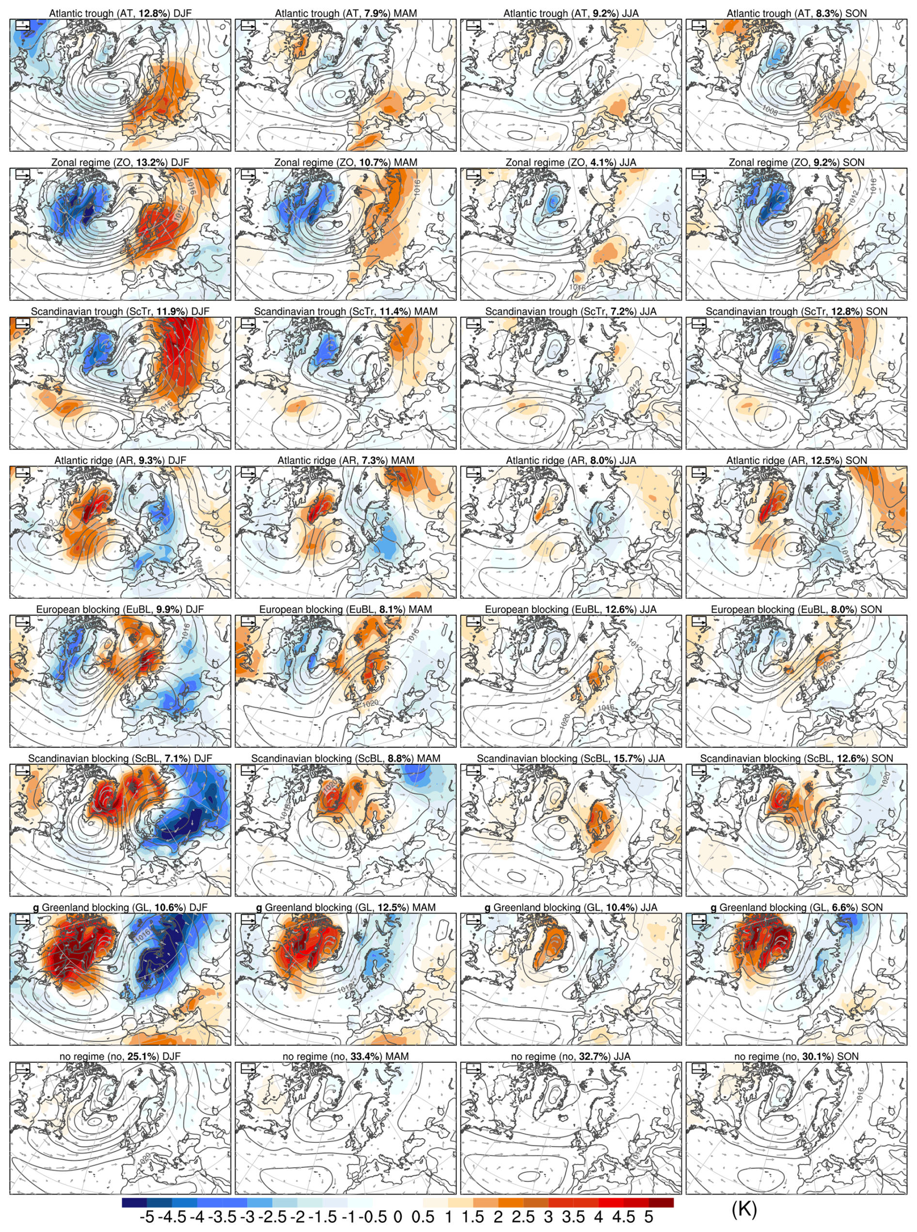
Figure 8 Composites of mean 2 m temperature anomalies (shaded every 0.5 K) during each of the regimes (rows) stratified according to season (columns). Anomalies are computed with respect to a 90 d running mean climatology and averaged for all days attributed to one of the seven or “no regime” in the respective three-months season (see Sect. 2). Contours show composite mean sea level pressure (every 4 hPa) and vectors 100 m wind with a reference arrow whose length corresponds to 8 m s⁻¹ wind speed to the top left. The regime name, abbreviation, seasonal regime frequency, and season are indicated in each panel caption.

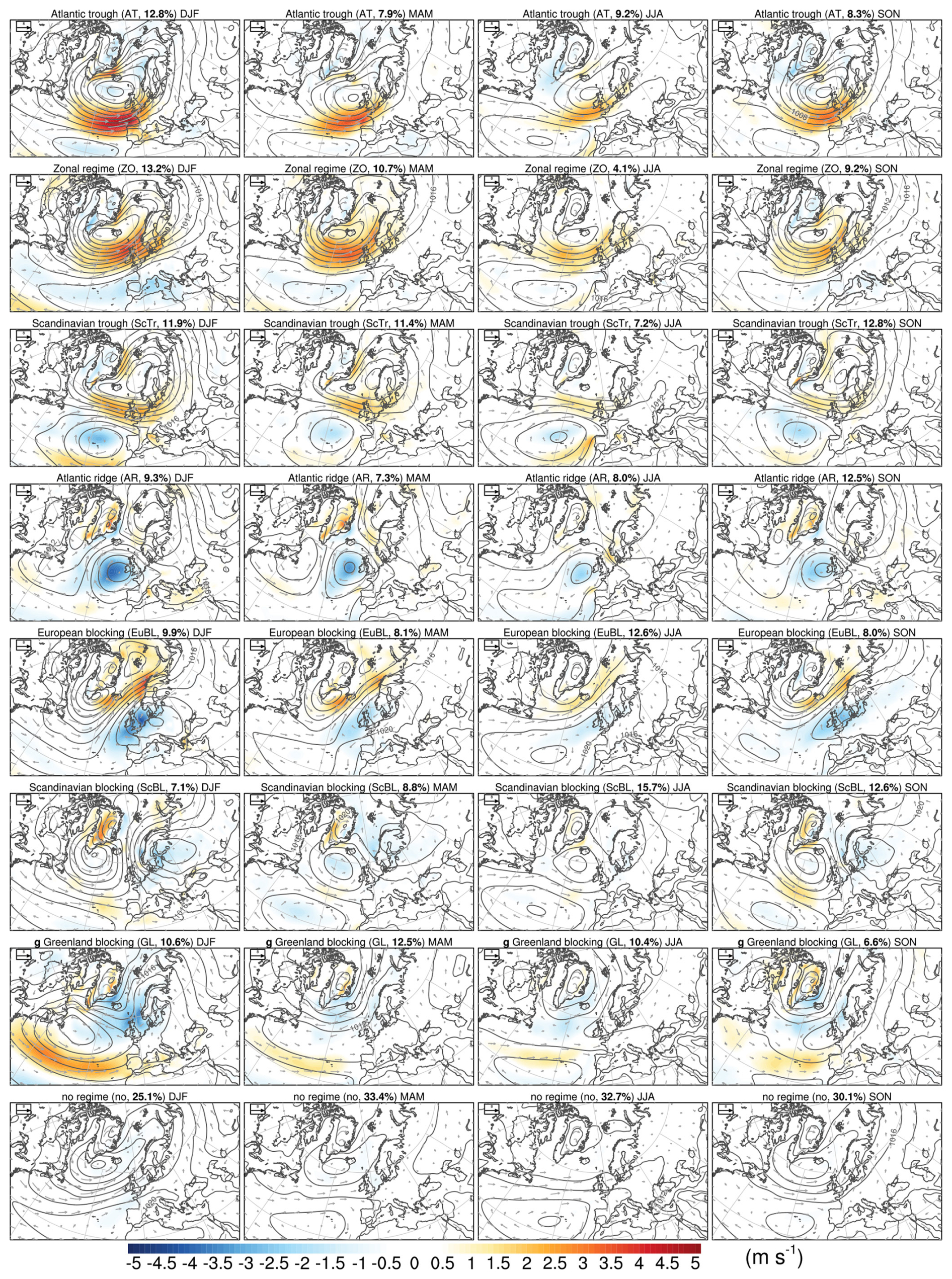
Figure 9 Composites of 100 m wind speed anomalies (shaded every 0.1 m s⁻¹) during each of the regime (rows) stratified according to season (columns). Anomalies are computed with respect to the seasonal climatology (see Sect. 2). Contours of mean sea level pressure and 100 m wind vectors as in Fig. 8.

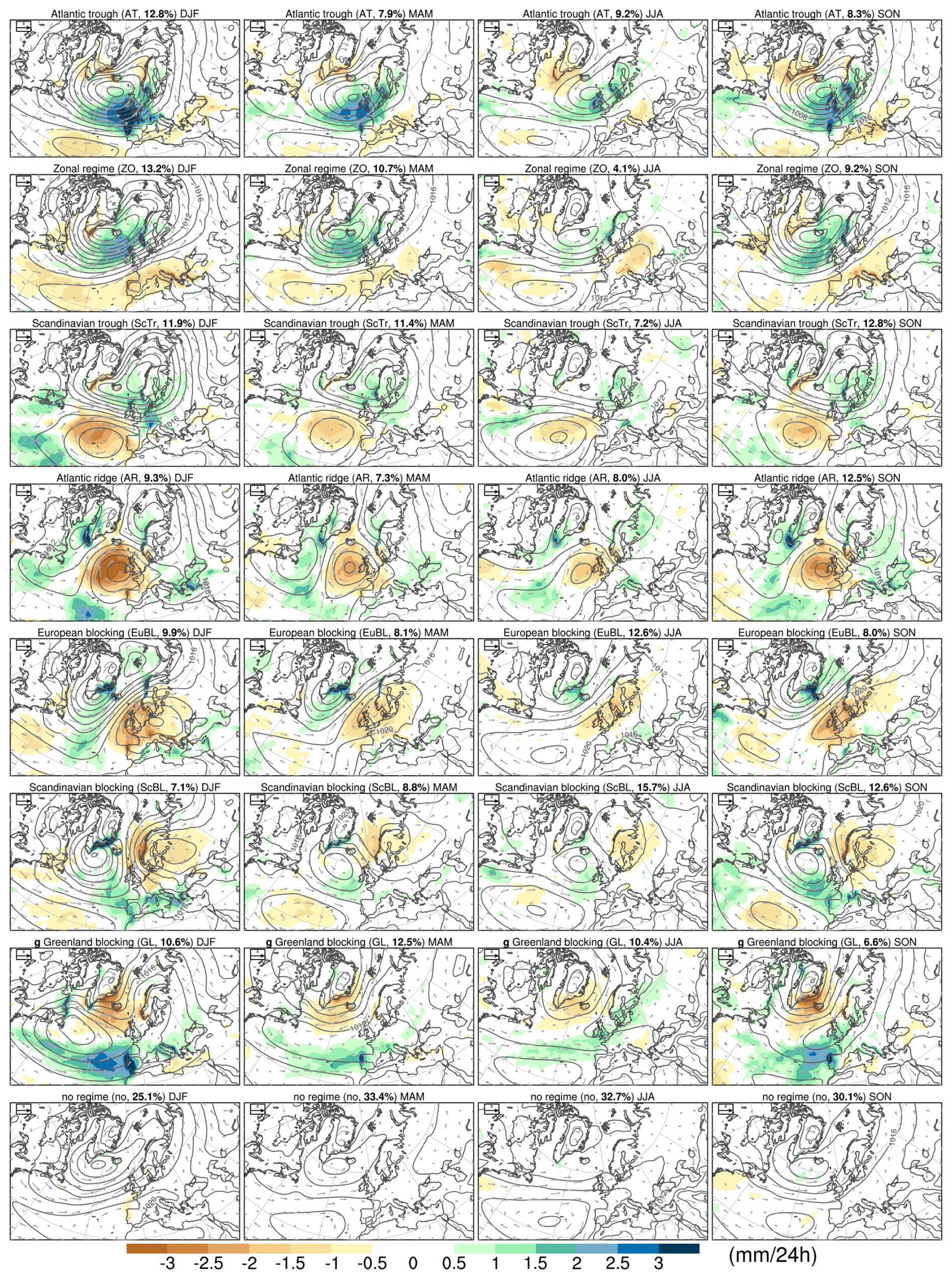
Figure 10 Composites of total precipitation anomalies (shaded every 0.5 mm 24 h⁻¹) during each of the regime (rows) stratified according to season (columns). Anomalies are computed with respect to the seasonal climatology (see Sect. 2). Contours of mean sea level pressure and 100 m wind vectors as in Fig. 8.

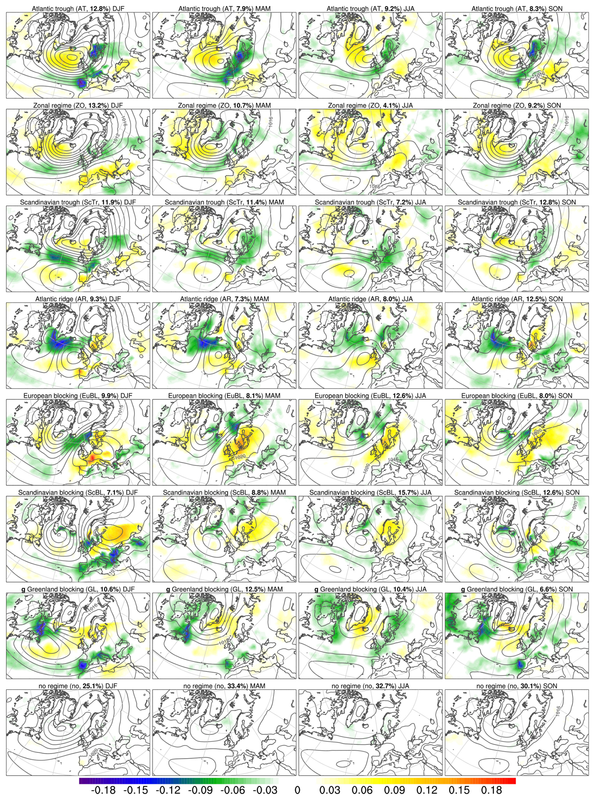
Figure 11 Composites of the anomaly in the daily fraction of incoming solar radiation (shaded in %) during each of the regime (rows) stratified according to season (columns). Anomalies are computed with respect to the seasonal climatology (see Sect. 2). Contours of mean sea level pressure and 100 m wind vectors as in Fig. 8.

5.4.1 2 m temperature

Generally speaking the cyclonic AT, ZO, and ScTr regimes feature anomalous warm conditions in most part of Europe with some regional variation. This is particularly pronounced in winter due to warm air advection ahead of strong surface cyclones (Fig. 8, 1st column, rows 1–3). However, ScTr in spring, summer, and autumn tends to go along with weak cold anomalies in Europe (Fig. 8, row 3). In contrast, the blocked regimes come along with cold conditions in many parts of Europe in winter, with variation according to the position of the surface high pressure system (Fig. 8, 1st column, rows 4–7). In other seasons AR and GL tend to feature moderately cooler than normal conditions in Europe, and warmer than usual conditions in Greenland, whereas EuBL and ScBL come along with warmer than usual conditions in most parts of Europe (Fig. 8, 2nd–4th column, rows 4–7). The ZO, EuBL, and ScBL regimes are prone for heat waves in different regions in summer (see Supplemental Fig. S2 in Spensberger et al., 2020). “No regime” days are close to climatology (Fig. 8, row 8).

5.4.2 100 m wind speed

The cyclone activity during AT, ZO, and ScTr also comes along with above average wind speed in western and central Europe (Fig. 9, 1st column, rows 1–3). The highest wind speed occurs on the southern flanks of low pressure systems. In contrast, the blocked regimes feature below average wind speed in countries adjacent to the North Sea region and western Europe with some variation depending on the regime (Fig. 9, 1st column, rows 4–7). Importantly, regions with below average wind speed are accompanied with above average wind speed at the flanks, e.g. over northern Scandinavia during EuBL, Iberia during GL, and the Mediterranean during AR. These patterns hold in other seasons, but with weaker magnitude. The impact of surface weather modulation during the seven regimes on wind power output and how knowledge about regime patterns can be used to balance pan-European wind power output has been extensively discussed in Grams et al. (2017).

5.4.3 Precipitation

Weather regimes also go along with similar patterns in total precipitation as for wind (Fig. 10). The cyclonic regimes feature enhanced precipitation in western and central Europe (AT), Northern Europe (ZO), and Northern and Central Europe (ScTr). At the same time drier than usual conditions prevail in the Mediterranean (ZO) and Iberia (ScTr). During AR, western Europe is anomalous dry, while southeastern Europe receives above average precipitation. EuBL and ScBL go along with dry conditions in Central and Northern Europe, respectively. At the same time peripheral regions receive above average precipitation, in particular southern Europe during ScBL. During GL, above average precipitation prevails in Iberia and Western Europe, often accompanied by atmospheric river landfall. Also these patterns are similar across season. However, as the storm track is weaker and poleward shifted in summer, and precipitation is dominated by local convection, the signals are weaker in summer. Most importantly, the region affected by above average precipitation during GL shifts from Iberia to the countries adjacent to the North and Baltic Seas in summer. A more in-depth analysis of precipitation anomalies as well as the shift in likelihood of extremes and atmospheric river landfall are provided in Pasquier et al. (2019).

5.4.4 Insolation

The modulation of solar radiation at the surface is computed in terms of the relative change of the daily maximum possible insolation that is the fraction of accumulated daily insolation and the accumulated daily insolation clear-sky. Anomalies only range between ±20 % (Fig. 11) and regions affected are similar to those of precipitation anomalies. This reflects that insolation is strongly modulated by clouds. Most importantly, regions in the centre of high pressure systems receive above average insolation during regimes. However, as discussed in Grams et al. (2017), due to high intra-regime variability of clouds and insolation (cf. Gerighausen et al., 2024) and generally limited impact of low-frequency variability on the total insolation (Grams et al., 2017) I do not go into further details.

Finally it must be stressed, that in some regions there is a huge intra-regime variability in terms of the surface weather impact. Thus, the composite mean can only provide a first indication of the surface weather conditions in a certain region during a specific regime. I refer to Gerighausen et al. (2025) and Spaeth et al. (2024) for an in-depth analysis on intra-regime variability of surface weather and the accompanying plot catalogue in Gerighausen et al. (2024) for an overview of the robustness of the patterns.

6 Variability and trends in regime occurrence 1950–2024

The regime assignment and life cycle identification has been extended back to 1950 and until present using the backward and near real-time extension of ERA5 (Soci et al., 2024). The 1940s are omitted due to the scarce data assimilated in ERA5 (Bell et al., 2021; Soci et al., 2024). The long time series raises questions regarding trends in regime occurrence, the stability of the regime definition with respect to the data period considered, and regarding decadal variability in regime patterns.

This last results section discusses the implications of variability and trends in Z500 on regime identification and potential trends in regime occurrence, while other aspects are left for future work. In fact, Dorrington and Strommen (2020) and Dorrington et al. (2022a) provide a comprehensive discussion of decadal variability in regime patterns and argue for stable regime behaviour in the North Atlantic European region.

Instead, here I adopt the perspective of Fischer et al. (2025) and investigate long-term variability and changes in regime occurrence using the fixed set of regime patterns representative for 1979–2019. Thus, the anomalies are computed relative to the fixed 1979–2019 reference period and projected into the regime patterns representative of 1979–2019 in order to attribute individual time steps to regimes.

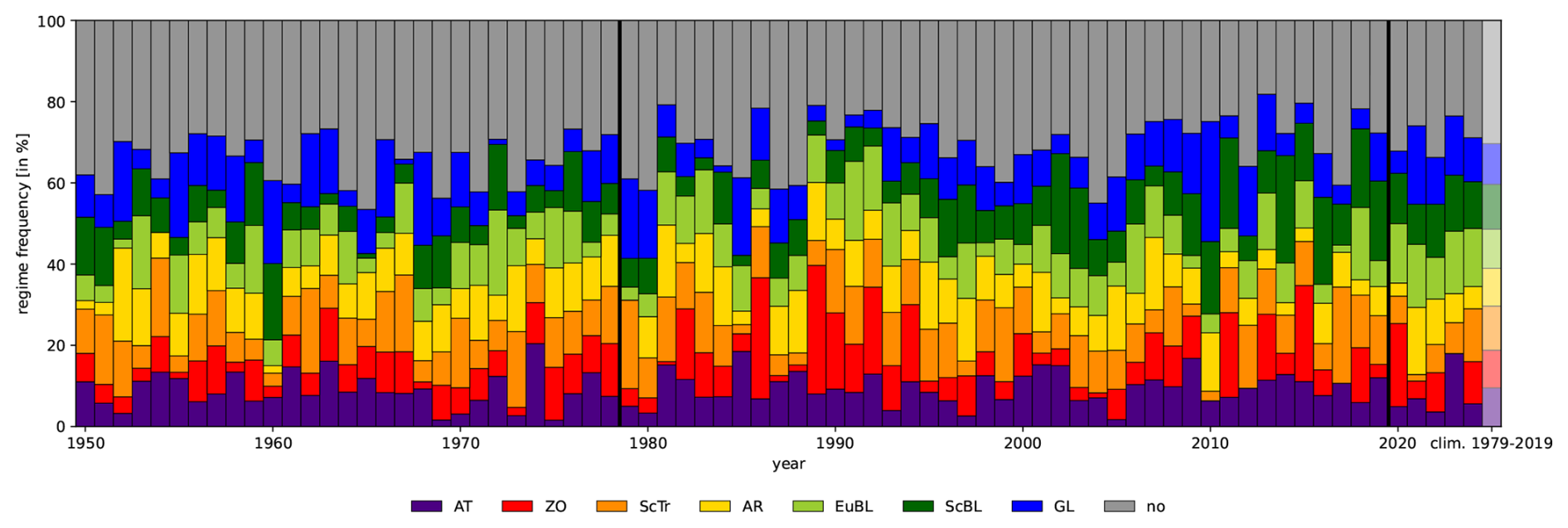
Figure 12 Inter-annual regime frequency in the extended data period 11 January 1950 until 31 December 2024. Stacked bars indicate the annual regime frequency for each year (in  %), the last, pale bar indicates the mean annual frequency for 1979–2019. The vertical bold lines separate the period 1979–2019 used for the regime definition, from the back- and forward extension 1950–1978 and 2020 until present.

Figure 12 shows the annual frequency of the regimes similar to Fig. 6c but from 1950 until 2024. Again the large inter-annual variability of regime occurrence is apparent also in the earlier decades 1950–1978. On a first subjective, visual inspection there is little evidence of marked decadal variability in regime occurrence, except for three periods of enhanced occurrence of cyclonic regimes (AT, ZO, ScTr) from 1961–1968, 1974–1979, and in the early 1990s (1989–1994). Another signal sticks out: an increase in the occurrence of blocking over the European region since the 1990s namely an increase in ScBL frequency (dark green).

6.1 Implications of geopotential height variability and trends

Before presenting results from a simple linear trend analysis, I discuss the potential effect of a global trend in Z500 on the regime identification. Various studies showed a good suitability of ERA5 (and other reanalysis data sets) for the study of global, and large-scale trends with mostly consistent signals across different data sets and in agreement with observations (Bell et al., 2021; Simmons, 2022; Soci et al., 2024). Simmons (2022) reports a global increase in ERA5 500 hPa geopotential height in recent decades consistent with an expected thermal expansion of the troposphere due to global warming. This trend has a particular regional pattern and might affect the regime identification.

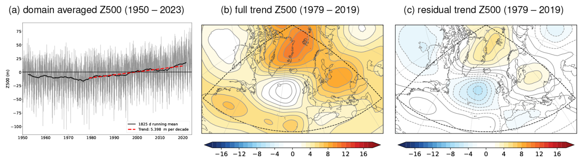
Figure 13 Trends in 10 d low-pass filtered 500 hPa geopotential height anomalies (units are gpm (10 yr)⁻¹). (a) Time series of spatial average in the EOF domain (80° W–40° E, 30–90° N) for 24-hourly time steps from 11 January 1950 until 31 December 2023 (grey) and 5-year running mean (black bold), as well as linear trend (red dashed) in the period 1 January 1979–31 December 2019. (b) Grid point based full trend (shaded every 1 gpm (10 yr)⁻¹) during the period 1 January 1979–31 December 2019. (c) Residual trend (shaded every 1 gpm (10 yr)⁻¹) computed by subtracting the area-averaged trend from panel (a) of 5.398 gpm (10 yr)⁻¹ from the full trend in panel (b).

The following replicates these trends with a focus on the domain and period used for the regime definition. Figure 13a shows the time series of the area-averaged 10 d low-pass filtered 500 hPa geopotential height anomaly. The 5-year running mean shows a very weak negative trend from 1950 to 1980. From 1980–present a first-order positive linear trend is apparent. In the following I focus on the period 1979–2019 used for the regime definition. In this period the linear trend equals 5.398 gpm (10 yr)⁻¹. A map of the grid point based full trends, reveals the regional pattern (Fig. 13b). While mostly positive, the increase in Z500 reaches up to 10 gpm (10 yr)⁻¹ over the Arctic, and remains enhanced over Scandinavia and eastern Europe as well as in the subtropical North Atlantic, whereas there is hardly any increase between Newfoundland and the British Isles. Recalling that the mean Z500 anomalies associated with the regimes are of an order of 𝒪(100 gpm), the trends in Z500 are an order of magnitude smaller (𝒪(10 gpm)). This means that deviations from mean conditions imposed by the intra-seasonal variability due to weather regimes is still larger than deviations arising from a potential trend in Z500. Therefore it is unlikely that trends affect the overall regime pattern.

Still, recent regime studies detrend Z500 anomalies in a simple manner by subtracting the area-averaged trend (Fig. 13a) from the full Z500 field (cf. Dorrington et al., 2022a; Lee et al., 2023). This accounts for the thermal expansion of the troposphere while retaining Z500 trends arising from circulation changes; i.e. changes in regime occurrence. Lee et al. (2023) called the trend that remains after subtracting the area-averaged trend from the full-trend as the “residual trend” (Fig. 13c). However, the determination of the “true” area-averaged trend is not straight-forward. Figure 13a shows that this first-order linearity assumption is only valid for the second half of the period and very sensitive to the choice of the data period. E.g. computing a linear trend of Z500 for 1979–2023 instead of 1979–2019 yields a trend of 5.996 gpm (10 yr)⁻¹ whereas computing it for 1950–2023 yields 3.334 gpm (10 yr)⁻¹ (not shown).

Here the residual trend is computed by subtracting the area-averaged linear trend 1979–2019 of 5.398 gpm (10 yr)⁻¹ from the local full-trend at each grid point (Fig. 13c). As expected the spatial pattern is retained. The residual trend shows a weak positive signal at high latitudes of the regime domain with a maximum of up to 5 gpm (10 yr)⁻¹ over the Arctic Seas, and a secondary maximum up to 3 gpm (10 yr)⁻¹ over Eastern Europe. Conversely a decreasing residual trend of up to −6 gpm (10 yr)⁻¹ is evident in the central North Atlantic, and weaker over Canada and the western Mediterranean. The question remains if the overall trend affects the regime identification.

Therefore, the regime identification has been repeated using detrended Z500 data for the computation of EOF-clustering, I_wr and regime life cycles. The detrending has been achieved by subtracting the area-averaged trend since 1 January 1979 accumulated until the given date from the Z500 fields at each grid point (assuming the linear trend of 5.398 gpm (10 yr)⁻¹ for 1979–2019; cf. Dorrington et al., 2022a; Lee et al., 2023).

The detrending has a marginal effect on the regime patterns and attribution of individual time steps (Figs. C6, C7). For all regimes, more than 95 % of the time steps contribute to the same EOF clusters as for the original regime definition, where no detrending has been applied (Fig. C7a). Similarly, regime life cycles contain at least 90 % of the same time steps in either configuration (Fig. C7b). The remaining 10 % of the time steps swap between related regimes and no regime – a sensitivity expected in the life cycle definition in particular for the precise (in terms of 3-hourly time steps) onset and decay phase of a life cycle (cf. Appendix B). The regime patterns themselves show hardly any difference (Fig. C6).

In conclusion, the current (1979–2019) global trend of Z500 hardly influences the regime identification, yet. Therefore, using either detrended or non-detrended data is not critical for most regime-related applications.

6.2 Trends in regime occurrence

It remains to investigate if there are significant trends in the occurrence frequency of regimes. To this end linear trends in regime occurrence are computed for both: the original and detrended ERA5 regime definition.

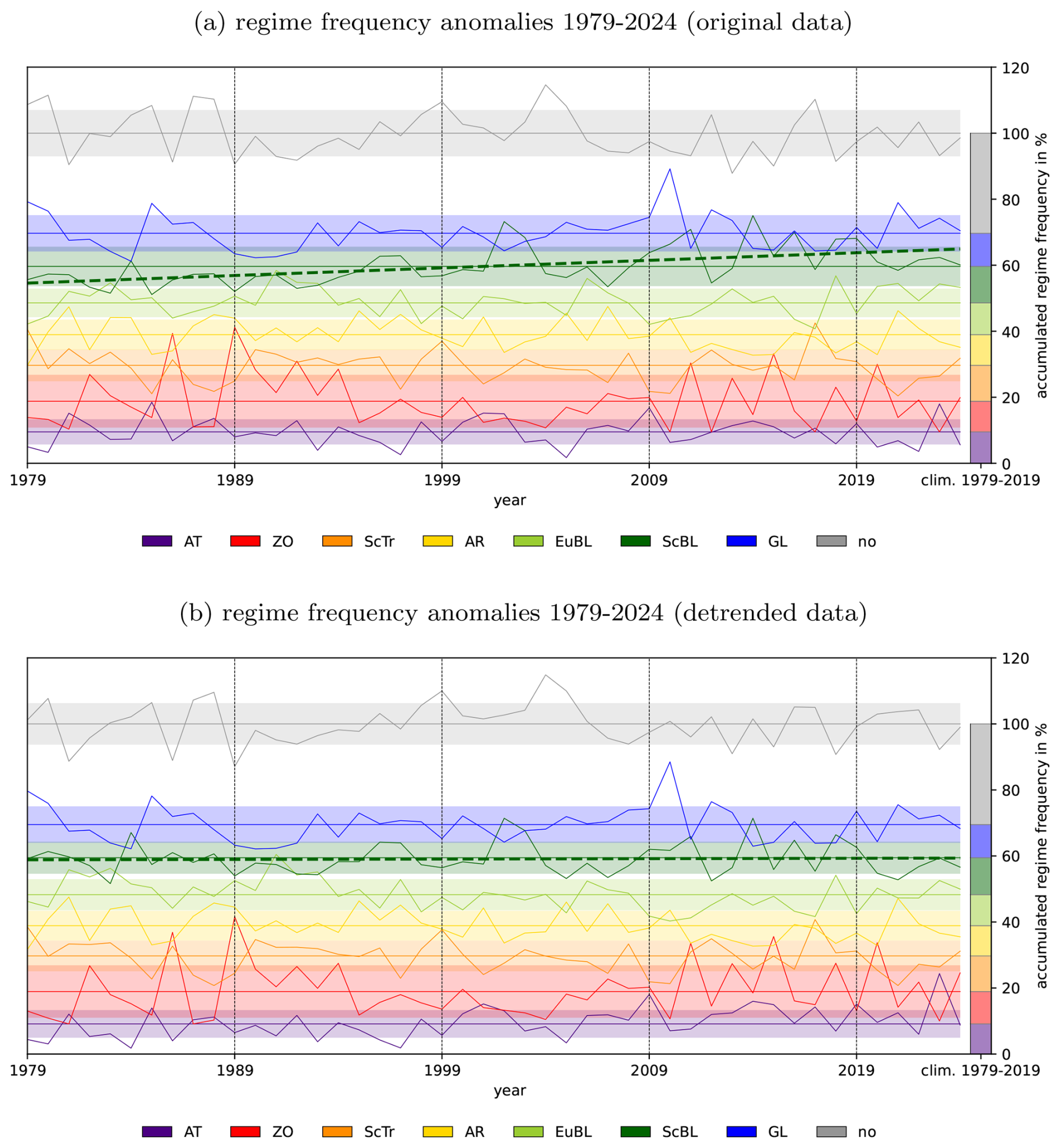
Figure 14 Anomalies of annual regime frequency (solid thin lines in  %) relative to the climatological mean occurrence frequency 1979–2019. The climatological mean frequencies are shown on the right as stacked bar as well as stacked thin horizontal lines. These serve as the reference for the illustration of the anomaly. In addition, the significant linear trend for ScBL is shown as a dashed dark green line. Shading denotes ±1 standard deviation of annual regime frequencies 1979–2019 centred around the respective climatological mean. (a) Data for the original ERA5 regime definition, and (b) for the variant using detrended Z500 (see text for details). Data shown for 1979–2024.

Figure 14 shows the anomalous annual regime frequency for the years 1979–2024 in a stacked visualisation with respect to the mean frequency. Tests with a simple linear trend analysis reveals huge sensitivity of trends to the length of the period considered. Significance has been tested with bootstrapping including FDR (false discovery rate) correction. Key results are summarized in the following. For the original data a significant trend in annual occurrence frequency can only be detected for blocking over Scandinavia (ScBL, Fig. 14a), consistent with the regional increase in Z500 due to thermal expansion (Fig. 13a, b). However, quantitatively trends vary markedly depending on the period used for trend calculation (1979–2019: 3.1 %, 1979–2022: 2.5 %, 1979–2024: 2.3 %). Furthermore seasonal trends vary even more and significance for seasonal trends emerges or disappears if the period for trend estimation is extended to 2024 or not. Still seasonal trends indicate that the annual trend is primarily driven by summer and autumn (ranging from 5.6 % to 6.7 % in summer, and from 2.3 % to 3.8 % in autumn). In contrast, in the detrended regime variant, excluding the thermal expansion of the troposphere in a simple manner, no significant trend can be detected. Still, the linear trends vary in a similar range, as for the original definition, if the period for linear trend analysis is altered.

Thus, there are two main conclusion from this simple trend analysis: (1) Internal variability in regime occurrence likely dominates over potential trends and the data period is too short for a robust assessment of trends with a simple linear trend analysis. (2) Detrending does not affect the regime patterns and gives helpful insight in the interpretation of trends. The significant trend in ScBL, which predominantly occurs in summer, is not present in a variant of regimes which are detrended accounting for the thermodynamic expansion of the troposphere in a simple manner. This suggests, that the reported trend in blocking in recent years, is likely primarily due to the thermodynamic effect of global warming and the detection method used, rather than due to a change in atmospheric circulation. Notwithstanding, overall higher geopotential height and temperatures likely amplify the local impact of blocking in terms of surface weather, in particular with respect to summer heat waves (Pfahl and Wernli, 2012; Chan et al., 2022). This raises the almost philosophical question of what to consider as blocked regime in a warmer climate: a circulation anomaly that deviates from the climatological background, or a region of very high pressure with strong impact on surface weather, in particular heat waves in summer? For the latter – impact-oriented perspective – the results shown here suggest that the thermodynamic effect of global warming alone can already partly explain the recent increase in episodes of high pressure in summer, reported in some studies, which a focus on circulation changes via a simple detrending would mask out.

Future work should explore the effect of a non-stationary climate on regime identification in a more sophisticated manner. It is difficult to justify linear detrending of Z500 due to the non-linearity in trends in Z500 (Fig. 13a). Instead a detrending for computing anomalies with respect to a “current climate mean” is needed. The LOESS filter technique used by more and more European national meteorological services for the analysis of trends in 2 m temperature allows such a disentangling of natural variability and climate change (Scherrer et al., 2023). Likewise the strong dependence of linear trend analysis to the period considered warrants caution for the interpretation of quantitative results and calls for methods suitable in a non-stationary climate, such as LOESS.

7 Summary

The study at hand provides a thorough documentation of a year-round weather regime definition for the North Atlantic European region. Together with the open release of data at Zenodo (Grams, 2025), it aims to be an entry point for the future work with these regimes. The definition has been first introduced by Grams et al. (2017) based on ERA-Interim. Small bug-fixes and the update to ERA5 make only marginal differences (Appendix B). Next to providing a short review of past studies based on the year-round regimes in the Introduction and an in-depth technical documentation (Sects. 2, 3, Appendix A) the study explores general characteristics of the year-round weather regime definition thereby revealing the following key novel insight:

1. The year-round regimes well cater for the 4 canonical seasonal regimes (Sect. 4). Moreover, the seven regimes reveal important variants and relationships between regimes: (a) there are two different types of blocking over the continent, EuBL and ScBL, with a slight preference for winter and summer, respectively. They still occur year-round and come along with different surface weather modultion. (b) A bimodal consideration of NAO positive/NAO negative episodes alone can be misleading as both can come along with cyclonic or blocked regime activity explained through the relationship of the ZO and EuBL/GL and AT regimes, respectively. (c) The AR regime is related to ScTr and EuBL but only the year-round definition carves out the actual ridge over the central Atlantic. (d) The GL (NAO negative) regime is relatively consistent across seasons.

2. There is some intra-annual and huge inter-annual variability in regime occurrence (Sect. 5.1). Only marginal signals of preferred regime transitions are detectable (Sect. 5.2).

3. The most extreme weather regime life cycles, i.e. life cycles lasting more than a month, co-occur with seasons characterised by extreme weather (Sect. 5.3), in line with the expected surface weather during a regime (Sect. 5.4).

4. Inter-annual variability in regime occurrence is high compared to potential trends (Sect. 6): a simple linear trends suggests a recent increase in the occurrence of Scandinavian blocking, primarily in summer and autumn. However, the trend is highly sensitive to the period considered and vanishes if the mean trend in geopotential height is removed prior to regime identification. This indicates that the frequency change in ScBL is likely not due to a circulation change but related to the thermal expansion of the tropopshere under global warming.

8 Concluding discussion

The high sensitivity of simple linear trend analysis warrants caution in trend estimates of weather regimes and in the interpretation of circulations changes in a warming climate. Some of the detected signal might be related to inter-annual and decadal variability in regime occurrence (Dorrington and Strommen, 2020) and is therefore sensitive to the period considered. Another part might be related to the thermal expansion of the troposphere. This raises the question of how to consider a non-stationary background state in regime identification and opens an interesting avenue for future research. E.g. defining regimes with geopotential height anomalies computed with respect to the current climate mean in a non-stationary climate by applying a LOESS filter (Scherrer et al., 2023), might allow to better disentangle already existent thermodynamic and circulation changes.

The novel aspect of regime life cycles enables manifold studies, focussing on regime impacts, physical processes, or sub-seasonal predictability. For example, Hauser et al. (2023a) showed that serial clustering of winter storms happens in the middle of well-established and long-lasting life cycles of cyclonic regimes rather than cyclone clustering would trigger a regime. Likewise Mockert et al. (2023) showed that cold Dunkelflauten are embedded in particularly long-lasting Greenland blocking life cycles. Both, long-lasting cyclonic regimes as well as long-lasting Greenland Blocking, are favoured during anomalous states of the stratospheric polar vortex (cf. Beerli and Grams, 2019). With respect to process studies, Hauser et al. (2024), Teubler et al. (2023), and Hauser et al. (2026) worked out a nuanced view of the role of moist processes during the onset of blocked regimes. Büeler et al. (2021) and Osman et al. (2023) documented the overall sub-seasonal forecast skill for regimes and showed that different sub-seasonal forecasting systems struggle particularly in correctly predicting European Blocking. Focussing on life cycle stages, Wandel et al. (2024) could show that it is the misrepresentation of moist-processes related to the warm conveyor belt during regime onset that results in poor forecast skill for the European Blocking regime.

Here the classical approach of EOF pattern recognition combined with clustering has been used and expanded in order to circumvent caveats of the well-established 4 canonical seasonal regimes (Vautard, 1990; Michelangeli et al., 1995; Ferranti et al., 2015). Also other studies argue that more than four regimes are needed to better describe large-scale flow variability in the European domain. E.g. Falkena et al. (2020) propose six European regimes, but they focus on winter. More recent work explores the application of regime thinking for the application of specific phenomena. E.g. the concept of targetted circulation types (TCT) introduced by Bloomfield et al. (2020) showed that TCT explain more of the variability in country-aggregated renewable power output and demand than weather regimes. However, TCTs come with the caveat of being less grounded in physics. Likewise Dorrington et al. (2024a, b) introduced the concept of event-prone (weather) regimes (EPRs) and demonstrated their usefulness in terms of facilitating a storyline approach for forecasting extreme events. In the era of AI, modern machine learning (ML) and AI methods are applied for pattern recognition and open new avenues for regime studies. For example, Spuler et al. (2024) investigated dynamical drivers of extreme precipitation in Morocco. They showed how AI can be used in order to tailor regime identification to a certain phenomena while retaining physical meaning in the regimes.

Regime thinking with a varied degree of complexity (i.e. the number of clusters considered) is particularly useful for condensing forecast information on the medium- and extended-range (sub-seasonal) forecast horizon (Grams et al., 2020). For short-term forecasting of the next 1–10 d the day-to-day weather variability is of utmost interest. For this forecast horizon weather pattern approaches are suited, as they best represent variability on synoptic time scales. Tailored to the UK, Neal et al. (2016, 2024) demonstrate how weather patterns and weather regimes can be combined for seamless predictions. Thereby direct probabilistic forecasts of weather patterns are provided for shorter lead times and weather patterns are grouped into the larger regimes for longer lead times. Recently, Strommen et al. (2025) confirmed the usefulness of combined weather regime – weather pattern forecasts from a theoretical point of view. Gerighausen et al. (2025) tackled the problem of daily weather variability differently. She proposes using the continuous regime information provided by the weather regime index I_wr in order to interpret surface weather impact across lead times rather than relying on categorical regime thinking. Moreover, Mockert et al. (2025) developed an ML-based post-processing to elucidate the predictive signal in ensemble forecasts of I_wr thereby making use of the linkage of regimes to sources of sub-seasonal predictability such as the Madden-Julian-Oscillation.

Building on this body of knowledge, ECMWF and MeteoSwiss are currently working towards an operationalisation of the year-round North Atlantic European weather regimes for sub-seasonal forecasting and climate monitoring. This will not only facilitate easier access to real-time forecast information but also opens new ways for providing dynamical context in climate monitoring at National Meteorological Services (e.g. MeteoSchweiz, 2025).

Appendix A: Technical documentation of the year-round regime definition

In addition to the general overview and discussion of the technical implementation of the year-round regime definition in Sect. 3, I provide here a comprehensive technical documentation, with the aim to ensure reproducibility. The original code is implemented in NCAR's NCL V6.2.1 (NCL, 2014) and uses the netcdf and grib-handling software CDO (Schulzweida, 2023). Appendix B summarises the few changes in the regime definition compared to the initial version of Grams et al. (2017) and discusses similarities and differences.

A1 Definition of normalised Z500 anomalies

The regime definition roots in normalised, 10 d low-pass filtered anomalies of Z500 (subsequently abbreviated Z500^∗), computed with respect to a 90 d running mean climatology (1979–2019). The following explains the exact procedure to compute Z500^∗. Ultimately Z500^∗ is computed for the entire extended ERA5 period from 11 January 1950, 00:00 UTC until 30 June 2025, 21:00 UTC in 3-hourly time steps.

1. Computation of the mean $\stackrel{\mathrm{‾}}{X\left(t_{\mathrm{c}}\right)}$ at each 3-hourly calendar time t_c as mean over all years 1979–2019:

   $$\begin{array}{}\text{(A1)}& \stackrel{\mathrm{‾}}{X\left(t_{\mathrm{c}}\right)}={\displaystyle \frac{\mathrm{1}}{N}}\sum _{\mathrm{yyyy}=\mathrm{1979}}^{\mathrm{2019}}X\left(t\right),\end{array}$$

   N=41: number of years, t_c = <MMDD_HH> is the calendar time – meaning the “time of year” for a given month MM, day DD, and hour HH (in UTC), t = <YYYYMMDD_HH> every 3 h for the years (YYYY) 1979–2019. X(t) stands for the two-dimensional field of Z500 at a given time step t. 29 February is omitted. In leap years, the climatological data of 1 March is used for 29 February.

2. Computation of a “90-day”running mean on $\stackrel{\mathrm{‾}}{X\left(t_{\mathrm{c}}\right)}$ to yield the “seasonal 90-day running mean climatology 1979–2019” of Z500 for each calendar time t_c=<MMDD_HH> averaged over the years 1979–2019:

   $$\begin{array}{}\text{(A2)}& \begin{array}{rl}& {\stackrel{\mathrm{‾}}{\stackrel{\mathrm{‾}}{X\left(t_{\mathrm{c}}\right)}}}^{\mathrm{90}\mathrm{d}}={\displaystyle \frac{\mathrm{1}}{M}}\sum _{i=-\mathrm{1092}\mathrm{h}}^{\mathrm{1092}\mathrm{h}}\stackrel{\mathrm{‾}}{X(t_{\mathrm{c}}+i)},\\ & i\in [-\mathrm{1092}\mathrm{h},\mathrm{1092}\mathrm{h};\text{ every }\mathrm{3}\mathrm{h}],\end{array}\end{array}$$

   M=730: number of 3-hourly time steps in the 91 d period (1092 h = 45 d × 24 h $/$ d + 12 h).

   A 90 d running mean is chosen to cover the duration of a season (three months). In contrast to a simple seasonal mean (e.g. for all time steps in DJF) or a monthly mean, the running mean ${\stackrel{\mathrm{‾}}{\stackrel{\mathrm{‾}}{X\left(t_{\mathrm{c}}\right)}}}^{\mathrm{90}\mathrm{d}}$ at each calender time also correctly represents the seasonal cycle of the reference climatology. It also avoids arbitrary jumps that happen at the end/begin of a season or month when using a fixed climatology for a season or a month, which is important in considering anomalies year-round.

3. Computation of 3-hourly anomalies X(t)^′:

   $$\begin{array}{}\text{(A3)}& X^{\prime }\left(t\right)=X\left(t\right)-{\stackrel{\mathrm{‾}}{\stackrel{\mathrm{‾}}{X\left(t_{\mathrm{c}}\right)}}}^{\mathrm{90}\mathrm{d}},\end{array}$$

   where X(t) is the two-dimensional Z500 field at 3-hourly time steps with t = 19500101_00 to 20250630_21.

4. Low-pass filtering of anomalies X^′(t) using Lanczos filter weights (Duchon, 1979):

   $$\begin{array}{}\text{(A4)}& {\widehat{X^{\prime }\left(t\right)}}^{\mathrm{LF}}=\mathrm{LF}\left(X^{\prime }\right(t\left)\right).\end{array}$$

   A low-pass > 10 d is implemented with a filter width of N=161 time steps or 20 d (for 3-hourly data), reasonable for filtering out variability including the synoptic time scale and the filter width following recommendations being double the cut-off frequency.

So far standard procedures e.g. as in Michel and Rivière (2011) are applied. However, ${\widehat{Z{\mathrm{500}}^{\prime }}}^{\mathrm{LF}}$ has a specific seasonal cycle in its amplitude. Therefore regimes are commonly identified for a specific season (e.g. DJF, JJA or extended seasons NDJFM, MJJAS; see the Supplement of Cassou, 2008 for a discussion of the effect of seasonality on regime patterns in Europe).

For a year-round definition, however, an EOF analysis and fuzzy clustering of the raw ${\widehat{Z{\mathrm{500}}^{\prime }}}^{\mathrm{LF}}$ across all seasons would be dominated by winter when anomalies have higher absolute values and higher variability than in summer. Therefore, I normalize ${\widehat{Z{\mathrm{500}}^{\prime }}}^{\mathrm{LF}}$ to remove this seasonal variability in amplitude while preserving spatial patterns. This allows to focus on the spatial flow pattern in the anomaly field.

In brief, I divide at each grid point ${\widehat{Z{\mathrm{500}}^{\prime }}}^{\mathrm{LF}}$ by a calendar time dependent scalar (which is the same at all grid points) representing the climatological variability of the amplitude of ${\widehat{Z{\mathrm{500}}^{\prime }}}^{\mathrm{LF}}$ at the respective calendar time. The scalar is defined as the spatial average of the climatological “temporal 30-day running standard deviation” over all anomalies between 1979–2019 and achieved as follows:

1. Computation of the 30 d “running” temporal standard deviation in a time period of ±15 d around each calendar time: at each grid point and for each calendar time step t_c compute the standard deviation of ${\widehat{Z{\mathrm{500}}^{\prime }}}^{\mathrm{LF}}$ over all the time steps t taken from a 30 d period around that calendar time (t_c−15 d < t < t_c+15 d) in all of the years (1979–2019).

2. Computation of the scalar normalisation weights: for each calendar time compute the area-weighted spatial average of this “temporal 30-day running standard deviation” in the EOF domain (see later).

3. Normalisation: divide ${\widehat{Z{\mathrm{500}}^{\prime }\left(t\right)}}^{\mathrm{LF}}$ by the normalisation weight for the respective calendar time. As for the EOF-clustering, the normalisation weights are computed using 6-hourly data for computational efficiency. For normalising time steps in between, the previous weight is used, e.g. for a 03:00 UTC time step the weight of the previous 00:00 UTC time step. This has no effect on the results.

Figure A1 illustrates the normalisation weights. The weights are higher in winter compared to summer reflecting the higher variability and amplitude of ${\widehat{Z{\mathrm{500}}^{\prime }}}^{\mathrm{LF}}$ in winter than in summer (Fig. A1a). The additional spatial maps show snapshot for winter (1 January, 00:00 UTC) and summer (1 July, 00:00 UTC; Fig. A1b) in the domain used for spatial averaging. The seasonal varying scalar weights results in the intended stronger normalisation in winter than in summer, and thus, a removal of the seasonal variability in amplitude of ${\widehat{Z{\mathrm{500}}^{\prime }}}^{\mathrm{LF}}$. In the following, I use the notion Z500^∗ for the normalised, low-pass filtered anomalies of Z500.

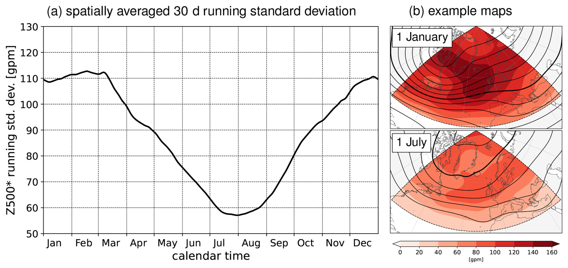
Figure A1 (a) Time series of the normalisation weight (y-axis) for each 6-hourly calendar time as the area-weighted spatial average in the domain 80° W to 40° E, 30 to 90° N of the “30-day running standard deviation” of ${\widehat{Z{\mathrm{500}}^{\prime }}}^{\mathrm{LF}}$ at each calendar time during 1979–2019. The x-axis shows the calendar time, with the 1st day of a month, 00:00 UTC marked by vertical lines. Units are geopotential metres (gpm). (b) Example maps of the “30-day running standard deviation” of ${\widehat{Z{\mathrm{500}}^{\prime }}}^{\mathrm{LF}}$ on 1 January, 00:00 UTC and 1 July, 00:00 UTC in the domain used for spatial averaging (shading, every 20 gpm). Contours show the 90 d running mean of Z500 (${\stackrel{\mathrm{‾}}{\stackrel{\mathrm{‾}}{Z\mathrm{500}\left(t_{\mathrm{c}}\right)}}}^{\mathrm{90}\mathrm{d}}$) every 80 gpm with the 5520 gpm isoline in bold.

A2 EOF analysis and clustering

Standard EOF analysis and fuzzy-c-means clustering identify the seven regime patterns. Key steps and the configuration used are repeated here.

First an EOF analysis is performed on 6-hourly Z500^∗ in the North Atlantic European domain 80° W to 40° E, 30 to 90° N and for the time period 11 January 1979, 00:00 UTC until 31 December 2019, 18:00 UTC². I use 6-hourly data instead of 3-hourly data for computational efficiency. However, 3-hourly data are used for the subsequent regime life cycles (Sect. A3). I tested the sensitivity to either 6-hourly, 24-hourly, or 48-hourly Z500^∗ as input for EOF-clustering and found no differences in the regime patterns (not shown). The choice of the domain follows previous studies using the same domain (Michel and Rivière, 2011; Dawson et al., 2012; Ferranti et al., 2015). In general, previous work on European weather regimes based on clustering showed only marginal sensitivity of the identified regimes on the exact choice (±10 deg) of the domain or configuration of the method (cf. Vautard, 1990; Michelangeli et al., 1995; Cassou et al., 2005; Cassou, 2008; Michel and Rivière, 2011; Cattiaux et al., 2013; Dawson and Palmer, 2015; Ferranti et al., 2015). The EOF analysis is computed with a standard implementation, here NCL (2014)'s function “eof_func”³.

Second, a fuzzy-c-means clustering (Bezdek, 1981) as in Harr et al. (2008) is performed in the phase space spanned by the leading seven EOFs (using an NCL implementation by Julian Quinting of the Matlab function dcfuzzy.m, https://de.mathworks.com/matlabcentral/fileexchange/9310-gui-for-multivariate-image-analysis-of-4-dimensional-data, last access: 7 August 2025). The seven leading EOFs explain 74.4 % of the variance. The EOF-clustering attributes each 6-hourly time step t unambiguously to one of the clusters by minimizing the intra- and inter-cluster distances in EOF phase space. Clustering is repeated, to test sensitivity to the random initial seeds and converged to the same clusters in each of the analysed setups. Thus, the clustering was insensitive to the initial seeds.

The clustering requires an a-priori choice of the number of clusters (= weather regimes). Seven clusters have been found to be optimal, as discussed in Sect. 4.1. I refer to these by the subscript wr with $\mathrm{wr}\in [\mathrm{AT},\mathrm{ZO},\mathrm{ScTr},\mathrm{AR},\mathrm{EuBL},\mathrm{ScBL},\mathrm{GL}]$ using the regime abbreviations introduced in the Introduction and explained in Sect. 4.

Finally, the mean regime pattern $\stackrel{\mathrm{‾}}{Z{\mathrm{500}}_{\mathrm{wr}}^{\ast }}$ according to the EOF-clustering is computed in geophysical space by averaging Z500^∗(t) of all 6-hourly time steps t attributed to a given cluster wr in the time period 11 January 1979, 00:00 UTC until 31 December 2019, 18:00 UTC.

A3 Objective identification of weather regime life cycles and life cycle stages

Inspired by pioneering work of Michel and Rivière (2011), the year-round regime definition newly introduces objective life cycles. The following presents the technical steps (Sect. A3.1–A3.3). Section 3.2 provides more information.

A3.1 Weather regime Index I_wr(t)

As in Michel and Rivière (2011), for each mean regime pattern $\stackrel{\mathrm{‾}}{Z{\mathrm{500}}_{\mathrm{wr}}^{\ast }}$ a weather regime index I_wr(t) is computed. I_wr(t) is defined as the normalised projection P_wr(t) of Z500^∗(t) into the cluster mean $\stackrel{\mathrm{‾}}{Z{\mathrm{500}}_{\mathrm{wr}}^{\ast }}$ at time step t. It is computed as follows:

1. Computation of the projection P_wr(t) time series for each weather regime:

   $$\begin{array}{}\text{(A5)}& \begin{array}{rl}{P}_{\mathrm{wr}}\left(t\right)=& {\displaystyle \frac{\mathrm{1}}{\sum _{(\mathit{\lambda },\mathit{\phi })}\cos \mathit{\phi }}}\sum _{(\mathit{\lambda },\mathit{\phi })}Z{\mathrm{500}}^{\ast }(\mathit{\lambda },\mathit{\phi },t)\\ & \cdot \stackrel{\mathrm{‾}}{Z{\mathrm{500}}_{\mathrm{wr}}^{\ast }(\mathit{\lambda },\mathit{\phi })}\cdot \cos \mathit{\phi },\end{array}\end{array}$$

   where the sums are over all grid points in the EOF domain (80° W–40° E, 30–90° N) given by the longitude, latitude coordinates λ,φ and $\mathrm{wr}\in [\mathrm{AT},\mathrm{ZO},\mathrm{ScTr},\mathrm{AR},\mathrm{EuBL},\mathrm{ScBL},\mathrm{GL}]$. This is done for all three-hourly time steps t in the time period 11 January 1979, 00:00 UTC until 31 December 2019, 21:00 UTC to yield a projection time series, and for each weather regime wr. Mathematically P_wr(t) is an unnormalised scalar measure for the correlation of Z500^∗ at any time t with the cluster mean regime pattern $\stackrel{\mathrm{‾}}{Z{\mathrm{500}}_{\mathrm{wr}}^{\ast }}$. As $\stackrel{\mathrm{‾}}{Z{\mathrm{500}}_{\mathrm{wr}}^{\ast }}$ are not normalized according to their amplitude, the absolute values of P_wr(t) markedly differ depending on the regime. Therefore, in the next steps P_wr(t) is normalised so that each wr gets equal weight when comparing projections.

2. Computation of the temporal mean $\stackrel{\mathrm{‾}}{P_{\mathrm{wr}}}$ of the projection time series P_wr(t) for normalisation:

   $$\begin{array}{}\text{(A6)}& \stackrel{\mathrm{‾}}{P_{\mathrm{wr}}}={\displaystyle \frac{\mathrm{1}}{N}}\sum _{\mathrm{1979}}^{\mathrm{2019}}{P}_{\mathrm{wr}}\left(t\right),\end{array}$$

   N is the number of 3-hourly time steps in the time period 11 January 1979, 00:00 UTC until 31 December 2019, 21:00 UTC.

3. Computation of the weather regime index time series I_wr(t) for each weather regime wr:

   $$\begin{array}{}\text{(A7)}& I_{\mathrm{wr}}\left(t\right)={\displaystyle \frac{P_{\mathrm{wr}}\left(t\right)-\stackrel{\mathrm{‾}}{P_{\mathrm{wr}}}}{\sqrt{\frac{\mathrm{1}}{N-\mathrm{1}}\sum _{\mathrm{1979}}^{\mathrm{2019}}{\left(P_{\mathrm{wr}}\left(t\right)-\stackrel{\mathrm{‾}}{P_{\mathrm{wr}}}\right)}^{\mathrm{2}}}}}.\end{array}$$

   The regime index is the standardised version of P_wr(t) (sometimes referred to as “standard score” of P_wr(t)), making comparable the regime projections for the different regimes. I_wr(t) is in units of standard deviation of P_wr(t) over the clustering period.

Ultimately, there are seven I_wr(t) time series for each of the seven regimes wr.

A3.2 Life cycle definition and life cycle stages

Michel and Rivière (2011) identified simple regime life cycles of 11 d duration by defining periods of monotonic increase and decrease of I_wr around a local maximum with fixed durations (7 d for monotonic increase, 4 d for monotonic decrease). They required that the 2 d period around the maximum belongs to the same regime according to the clustering and that I_wr>1.33 in that 2 d period. By definition, this allows overlapping regimes which makes physically sense, as e.g. processes fostering the onset of one regime might foster the decay of another while occurring at the same time.

Here I follow up the original idea of Michel and Rivière (2011) and expand it into an objective life cycle definition. The regime life cycle definition objectively identifies the time of the onset (on), decay (dc), as well as of the maximum projection (mx). The time of the start and end of a “saturation period” (st, se) are identified as auxiliary anchor points characterising the mature stage (period st : se) of a life cycle; but in practice this is only of technical relevance (see steps below). In addition times of regime transitions (tr) are identified (Sect. A3.3). The I_wr time series allows determining these life cycle stages in an objective manner. The following steps are performed for each regime wr:

1. Identification of the time step mx of the local maxima:

   The life cycle definition is centred around local maxima of I_wr(mx), $wr\in [\mathrm{AT},\mathrm{ZO},\mathrm{ScTr},\mathrm{AR},\mathrm{EuBL},\mathrm{ScBL},\mathrm{GL}]$. The construction of a life cycle begins by identifying candidates for I_wr(mx) fulfilling the following criteria:

   • a.

     I_wr(mx) is a local maximum, meaning for the time steps before and after mx the index is smaller:

     $$I_{\mathrm{wr}}(\mathrm{mx}-\mathrm{\Delta }t)<I_{\mathrm{wr}}\left(\mathrm{mx}\right)>I_{\mathrm{wr}}(\mathrm{mx}+\mathrm{\Delta }t).$$
   • b.

     I_wr(mx)>thres_abs: projection is larger than a minimum threshold (here thres_abs=1.0).

   • c.

     mx is not the first or last time step of the data period.

   • d.

     $\stackrel{\mathrm{‾}}{\mathrm{\Delta }{I}_{\mathrm{wr}}(\mathrm{mx}-\mathrm{\Delta }{t}_{\mathrm{pre}}:\mathrm{mx})/\mathrm{\Delta }{t}_{\mathrm{pre}}}>\mathrm{0}$ and $\stackrel{\mathrm{‾}}{\mathrm{\Delta }{I}_{\mathrm{wr}}(\mathrm{mx}:\mathrm{mx}+\mathrm{\Delta }{t}_{\mathrm{post}})/\mathrm{\Delta }{t}_{\mathrm{post}}}<\mathrm{0}$: an average increase/decrease of the projection must occur prior/after mx. Here Δt_pre and Δt_post are 5 d. The period is shortened if mx is close to the begin or end of the data period.

   Based on these mx candidate times, candidate times for on, st, se, dc are derived.

2. Computation of the time steps of the start and end of saturation period st, se:

   A saturation period centred around mx is defined. The begin st of this period is marked by the first time, when I_wr does no longer experience a strong increase: $\frac{\mathrm{\Delta }{I}_{\mathrm{wr}}\left(\mathrm{st}\right)}{\mathrm{\Delta }t}<{\left.\frac{\mathrm{\Delta }{I}_{\mathrm{wr}}}{\mathrm{\Delta }t}\right|}_{\mathrm{start}}$, where ${\left.\frac{\mathrm{\Delta }{I}_{\mathrm{wr}}}{\mathrm{\Delta }t}\right|}_{\mathrm{start}}>\mathrm{0.0}$ is a given threshold (here set to $\mathrm{0.2}/\mathrm{24}$ h and Δt=3 h). Likewise the end of the saturation period is defined as the last time, before I_wr experiences a strong decrease: $\frac{\mathrm{\Delta }{I}_{\mathrm{wr}}\left(\mathrm{se}\right)}{\mathrm{\Delta }t}>{\left.\frac{\mathrm{\Delta }{I}_{\mathrm{wr}}}{\mathrm{\Delta }t}\right|}_{\mathrm{end}}<\mathrm{0.0}$ (here set to $-\mathrm{0.2}/\mathrm{24}$ h and Δt=3 h).

   If I_wr becomes smaller than thres_abs or if it is no longer larger than a projection into another regime, the slope criteria are not imposed, and the first/last time when the latter criteria are valid are assigned for st $/$ se. The following relations are valid: $\mathrm{st}\le \mathrm{mx}\le \mathrm{se}$, $I_{\mathrm{wr}}(\mathrm{st}:\mathrm{se})>{\mathrm{thres}}_{\mathrm{abs}}$.

3. Determination of the time of weather regime onset on and decay dc:

   The onset (decay) of a weather regime life cycle is defined as the first (last) time when I_wr(on)>thres_abs (I_wr(dc)>thres_abs). The following relations are valid: $\mathrm{on}\le \mathrm{st}\le \mathrm{mx}\le \mathrm{se}\le \mathrm{dc}$.

4. Filtering through merging candidate life cycles:

   To avoid that life cycles of the same regime happen at the same time (which might occur if they anchor around different local maxima, but identify the same on, st, se, dc), weather regimes of the same wr are merged. In that case the earliest on, st, and latest se, dc times are attributed to the merger regime, and mx corresponds to the time, when I_wr is the maximum within the merged regime period. During a merger regime, changes of I_wr larger than the thresholds imposed for the computation of st, se may occur, but overall I_wr remains at a high level in the period st : se. A merger regime life cycle fulfils the following criteria (explained using two candidates, but also a found merged regime can become another merger candidate, while iteratively checking all candidates):

   • a.

     Maxima mx1, mx2 are merged if either they share the same st or/and se or if the mean $\stackrel{\mathrm{‾}}{I_{\mathrm{wr}}(\mathrm{mx}\mathrm{1}:\mathrm{mx}\mathrm{2})}\ge {\mathrm{thres}}_{\mathrm{abs}}$ is greater than the given threshold (here thres_abs=1.0),

   • b.

     maxima to be merged do not occur more than $\mathrm{\Delta }{t}_{\mathrm{mx}}>\mathrm{mx}\mathrm{2}-\mathrm{mx}\mathrm{1}$ days from each other (here Δt_mx=100 d) and the mean $\stackrel{\mathrm{‾}}{I_{\mathrm{wr}}(\mathrm{on}:\mathrm{dc})}\ge {\mathrm{thres}}_{\mathrm{abs}}$ (here thres_abs=1.0) from onset to decay of the merged life cycle is greater than the given threshold,

   • c.

     number of time steps t within (on : dc) with I_wr(t)≤thres_abs is at most the equivalent of 5 d.

   Finally, various filters are applied for further cleaning the data: First a minimum duration of a life cycle is imposed requiring ($\mathrm{dc}-\mathrm{on}\ge \mathrm{minduration}$, here minduration=5 d). Then it is checked, that during a life cycle I_wr(mx) of that life cycle is the largest of all I_w(mx), w≠wr or I_wr(t) is maximum of all I_w, w≠wr for a number of time steps t during (on : dc) equivalent to at least 5 d (not necessarily a consecutive period of 5 d), and at least for one time step during (on : dc) I_wr is by ΔI=0.5 larger than any other I_w, w≠wr or the fraction of times where I_wr is larger than all other I_w, w≠wr is larger than 1/3 of the entire life cycle duration on : dc.

   Admittedly, several of the choices made for criteria and thresholds seem arbitrary. However, the final setup has been defined after 1.5 years of subjective testing with various configurations and these choices have been continuously questioned in studies using the regimes. Over the years, the configuration turned out to be still the ideal setup for the many subsequent studies. Most importantly the final criteria and filtering out ensure unambiguity of life cycles, while avoiding leaving too many episodes with “no regime” where one would still expect a regime to happen.

A3.3 Definition of regime transitions

Identification of regime transitions: the time of a regime transition tr of regime w1 is defined as the time after regime decay dc when another regime life cycle w2 becomes the dominant active life cycle (I_w2(tr) is maximum of all other active life cycles I_w(tr), w≠w2). tr is allowed to occur up to 4 d after the decay of the previous regime, meaning $\mathrm{dc}\le \mathrm{tr}\le \mathrm{dc}+\mathrm{4}$ d. This is the definition of the transition time used in this paper and termed “decay to” dcto in the auxiliary data. Thus, it asks “What is the subsequent regime after regime decay?” Note that the transition is to “no regime” if there is no subsequent active life cycle.

Several other definitions have been tested, and are provided in the auxiliary data. I briefly explain these for completeness: A backward looking perspective asks similarly as above but “What was the regime before or at the time of the regime onset?”. It is termed “onset from” onfr, meaning $\mathrm{on}-\mathrm{4}\mathrm{d}\le \mathrm{onfr}\le \mathrm{on}$. An instantaneous regime transition does not allow for the other regime to occur within 4 d: “transition to” trto is the first time when the active life cycle is no longer dominant over another active life cycle (I_wr of the considered life cycle becomes smaller than the one of the other active life cycle); similarly “transition from” trfr is the first time when the current life cycle becomes dominant over another active life cycle.

Appendix B: Differences to the original definition based on ERA-Interim

The paper at hand provides an update and thorough documentation of the earlier introduced year-round European weather regimes of Grams et al. (2017) based on ERA-Interim reanalysis. For completeness I briefly explain key differences in the configuration and show quantitatively, that overall there are only marginal differences in the identification of regime life cycles and attribution of time steps to a specific regime due to the adopted changes in the regime definition and the switch to ERA5.

The following updates have been made in the regime definition based on ERA5 compared to ERA-Interim:

1. Data period covers 1979–2019 instead of 1979–2015.

2. Grid spacing of data used is 0.5° instead of 1.0°.

3. Normalisation weights use the latitudinally weighted spatial mean of the grid point-based “temporal 30 d running standard deviation” for ERA5. The ERA-Interim definition in Grams et al. (2017) did not use weighted averages to compute the spatial mean.

4. EOF analysis and clustering performed on 6-hourly data for both variants

5. I_wr, life cycles, and life cycle attribution computed for 3-hourly data instead of 6-hourly data

Differences might occur due to the (1) the change of the reanalysis data set, (2) the latitudinal weighting of the normalisation weights (which was missing in the original definition due to a bug), and (3) the extension of the data period from 2015 to 2019. The biggest differences arise from (2) and (3): The latitudinal weighting for the normalisation weights reduces the importance of the variability in amplitude at higher latitudes, resulting in slightly weaker normalisation weights in summer (see Fig. B1a). This improves the detection of regimes in summer (Fig. B1c, d). As a consequence, the occurrence frequency of “no regime” has less seasonality – an intended effect. However, overall there are hardly discernable differences in the regimes patterns (cf. Fig. B2). Only ScBL shows a slightly stronger positive Z500 anomaly over Scandinavia. This is likely influenced by the high frequency of ScBL in recent years (2015–2019, discussion in Sect. 6), and alters somewhat the sharpness of the ScBL pattern. Comparing the attribution of 6-hourly time steps in ERA-Interim to the same time steps in ERA5 according to the respective life cycle attribution almost all time steps are attributed to the same regime, independent of the choice of either definition. There are only two noticable differences: (1) About 0.9 % less “no regime” time steps (31.5 % in ERA-Interim vs. 30.4 % in ERA5). Time steps which were previously attributed to “no regime”, based on the initial ERA-Interim definition are now attributed to one of the seven regimes (Fig. B1b) – an intended effect due to the increase of the attribution of time steps in summer. (2) some time steps which were EuBL in ERA-Interim are ScBL in ERA5, and some time steps which were ScBL in ERA-Interim are AT or GL in ERA5 – an effect likely due to the sharper ScBL pattern in the extended data period. Remaining differences are marginal swaps between related regimes (see Sect. 4.3) and “no regime” times. Overall results hold independent of the choice of either regime definition and I recommend to use the refined definition based on ERA5 for future studies.

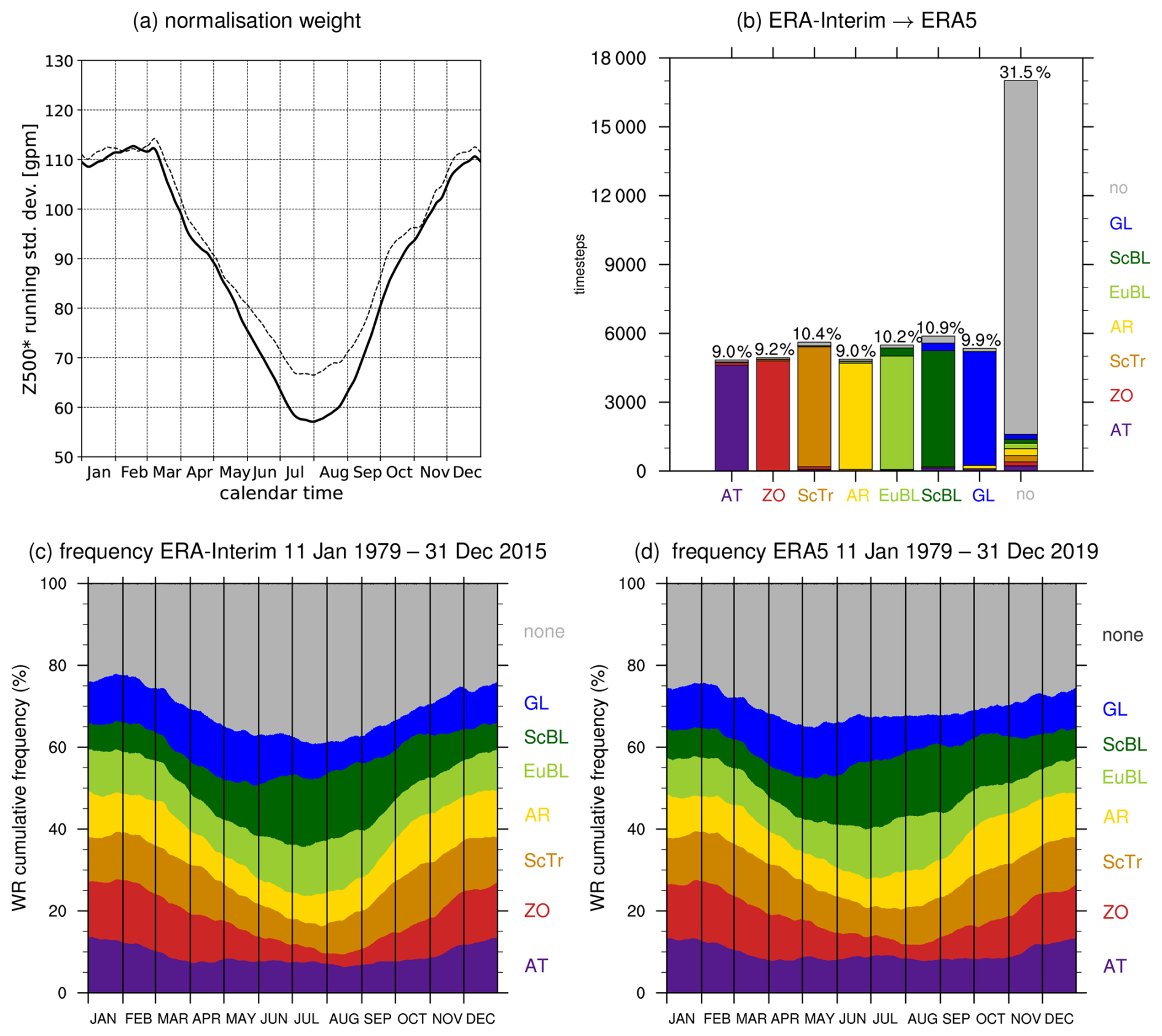
Figure B1 Comparison of the original year-round definition of Grams et al. (2017) based on ERA-Interim and the update on ERA5. (a) Scalar normalisation weights (in gpm) for normalising the low pass-filtered Z500 fields for ERA5 (solid, 1979–2019) and ERA-Interim (dashed, 1979–2015, computed without latitudinal weighting; cf. Fig. A1 and Sect. A1). (b) Life cycle attribution of six-hourly time steps (1979–2015) in ERA-Interim (x-axis) and ERA5 (coloured segments). Bars on the x-axis correspond to each of the 7 regimes and no-regime in ERA-Interim and are coloured by the fraction of regimes to which they are attributed in the ERA5 based definition. As in Fig. 6a, panels (c) and (d) show the intra-annual variability in regime frequency for the original ERA-Interim definition (c, 1979–2015) and the updated definition with ERA5 (d, 1979–2019).

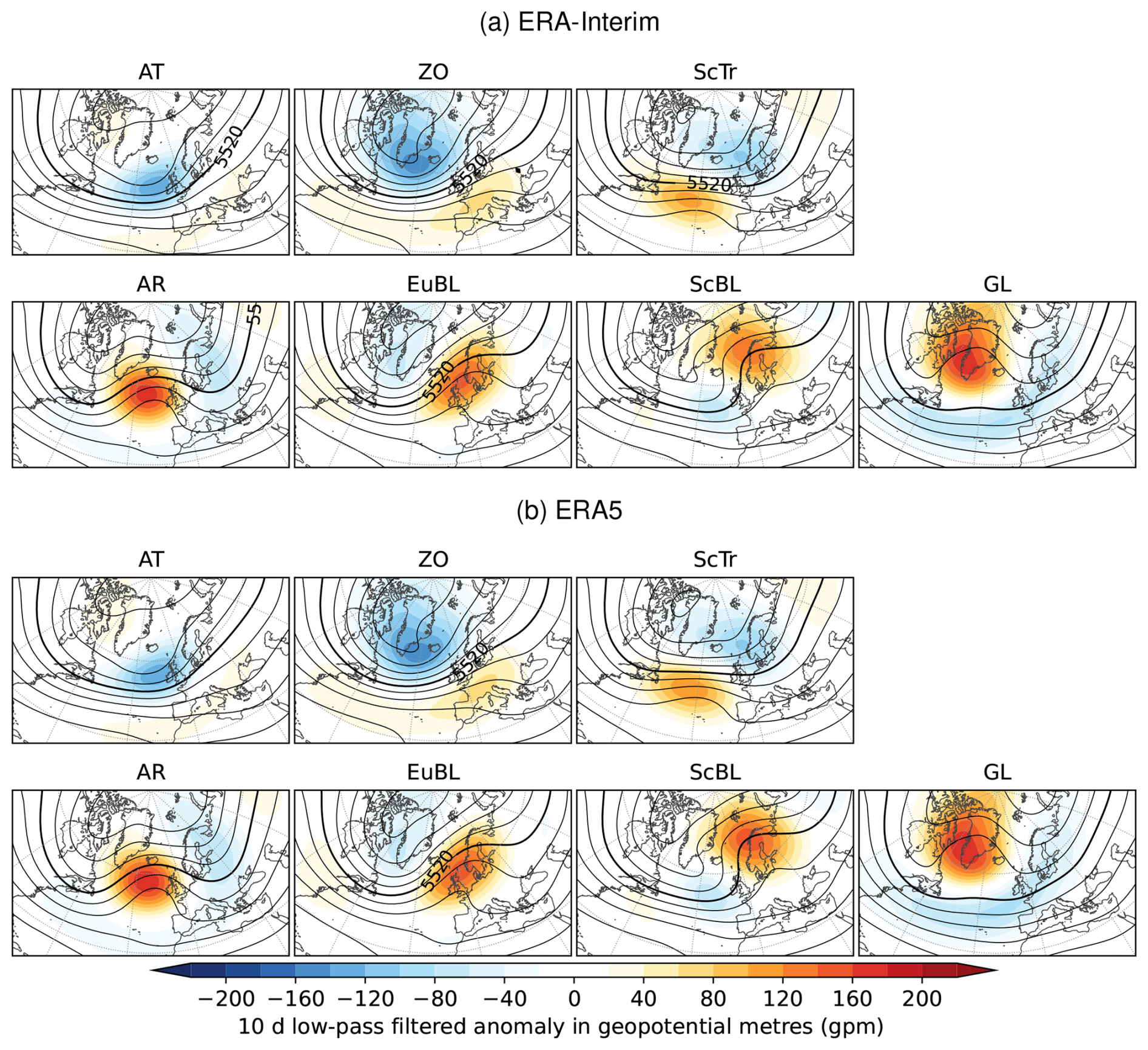
Figure B2 As in Fig. 2, cluster mean of low-pass filtered Z500 anomaly (shaded every 20 gpm) and absolute field (contours every 80 gpm, 5520 gpm in bold) based on the (a) ERA-Interim and (b) ERA5 definitions. The panel labels indicate the regime abbreviation.

Appendix C: Additional figures

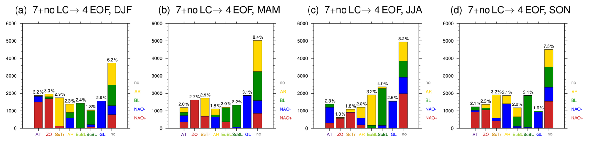
Figure C1 As Fig. 5 but vice-versa frequency of the year-round 7+1 regimes in each season and coloured bar segments indicate how these time steps correspond to the 4 seasonal regimes based on non-normalized data (1979–2019) for different seasons. Labels on x-axis indicate the regime name and colour code for the 7+1 regimes, labels to the right of each sub-figure indicate the name and colour-code for the 4 seasonal regimes.

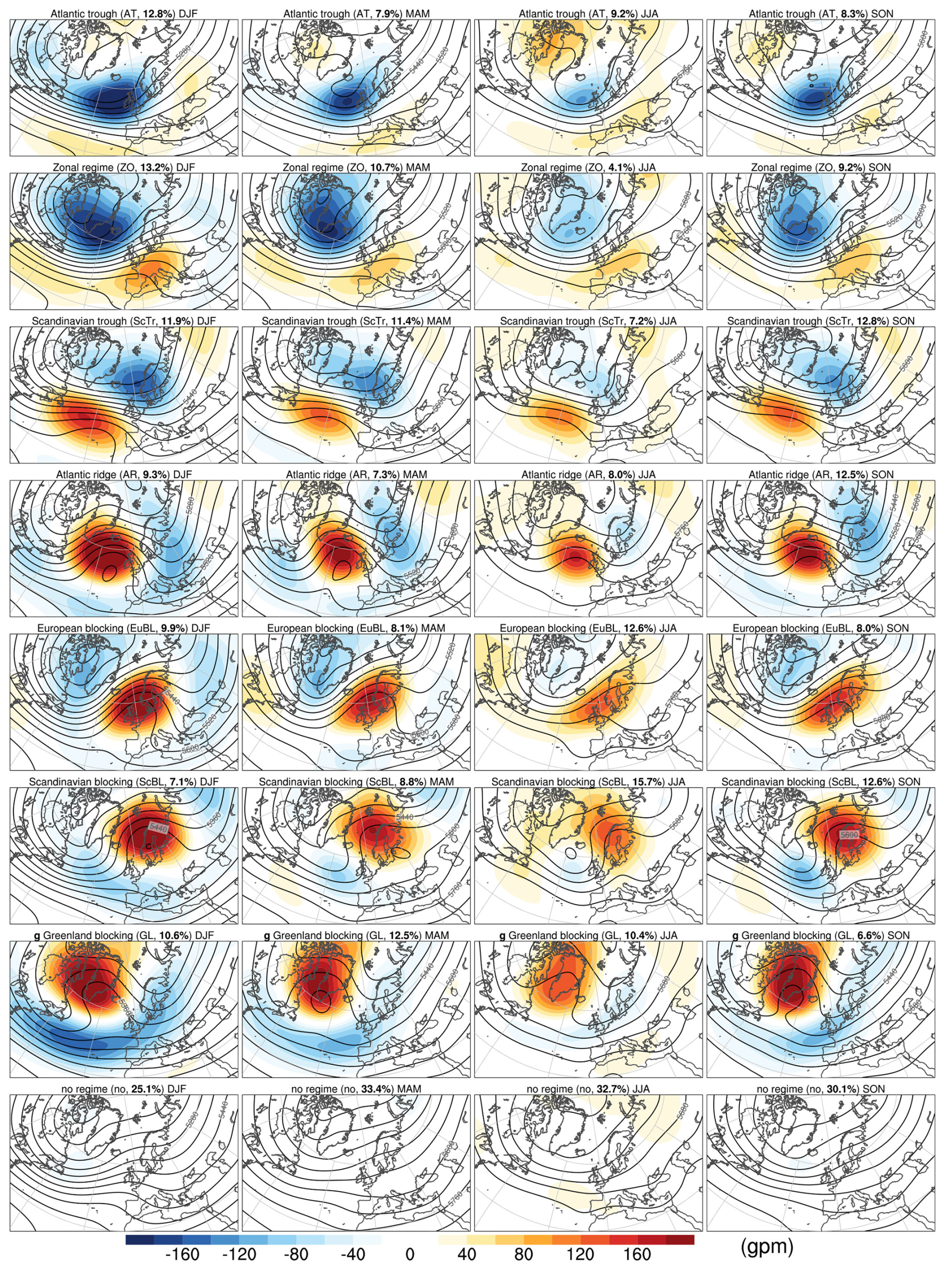
Figure C2 As Fig. 3 but stratified according to seasons.

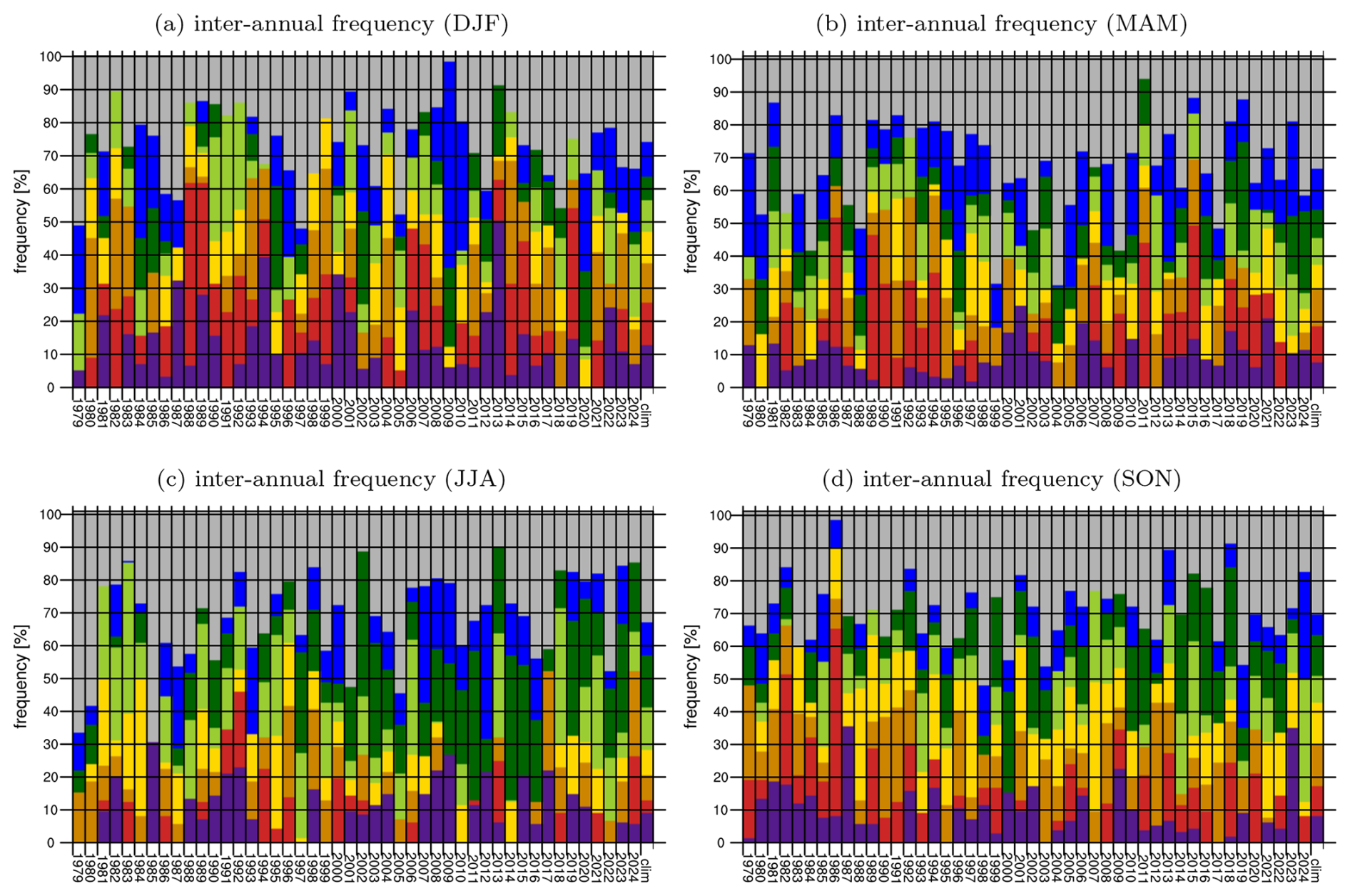
Figure C3 As Fig. 6b but for seasonal regime frequency in each year 1979–2024 (bars), and the climatological mean for comparison (right-most bar).

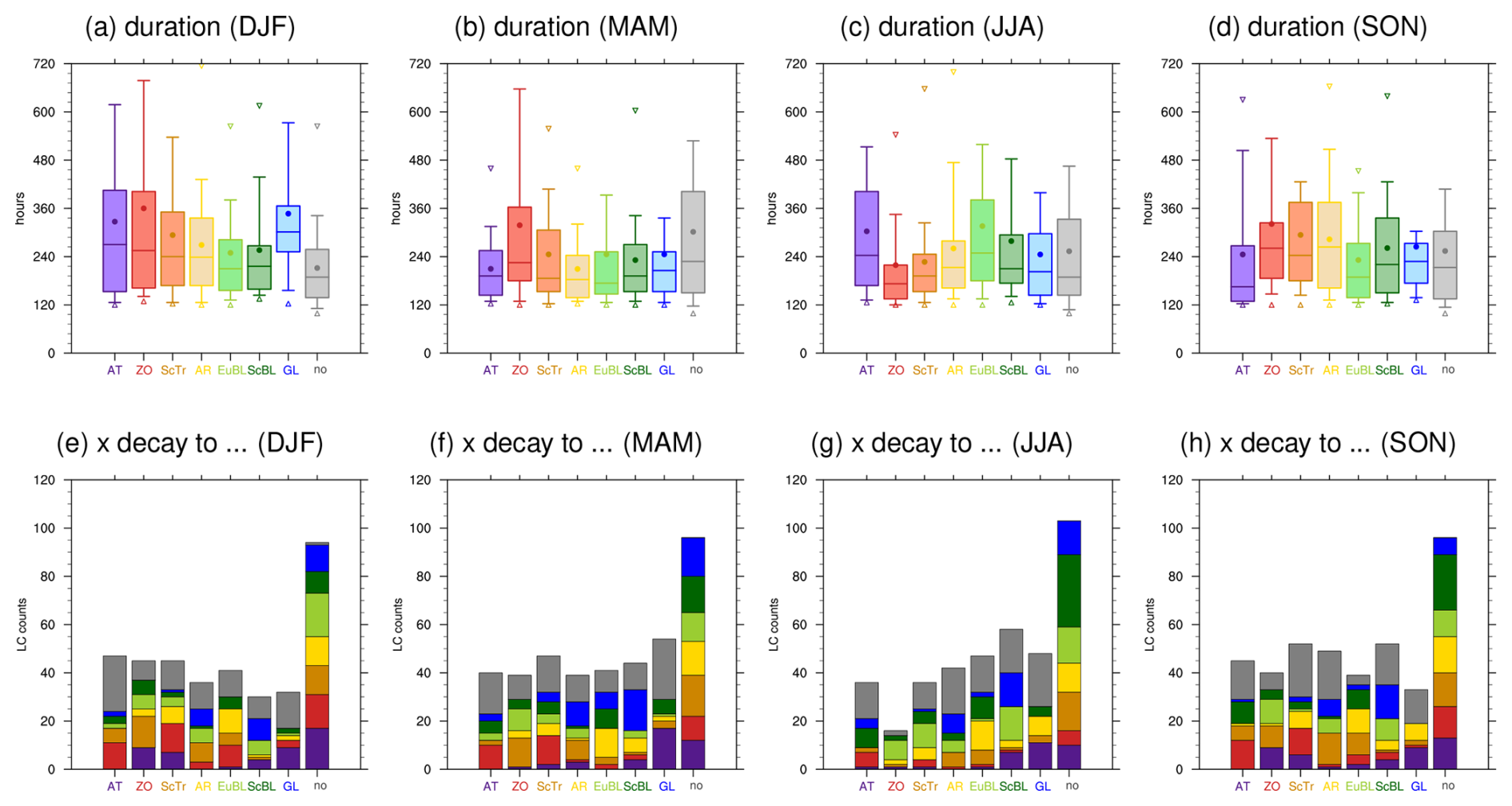
Figure C4 As Fig. 7 but stratified according to seasons. (a–d) Duration of regime life cycles, whiskers show the 10 % and 90 %, the box the 25 %, median, and 75 % percentile, respectively. Coloured dot shows the mean and the triangle the minimum duration. Bars in panels (e)–(h) show the number of life cycles for each regime (x-axis) and the coloured segments in each bar the number of transitions into other regimes within a 4 d period after decay.

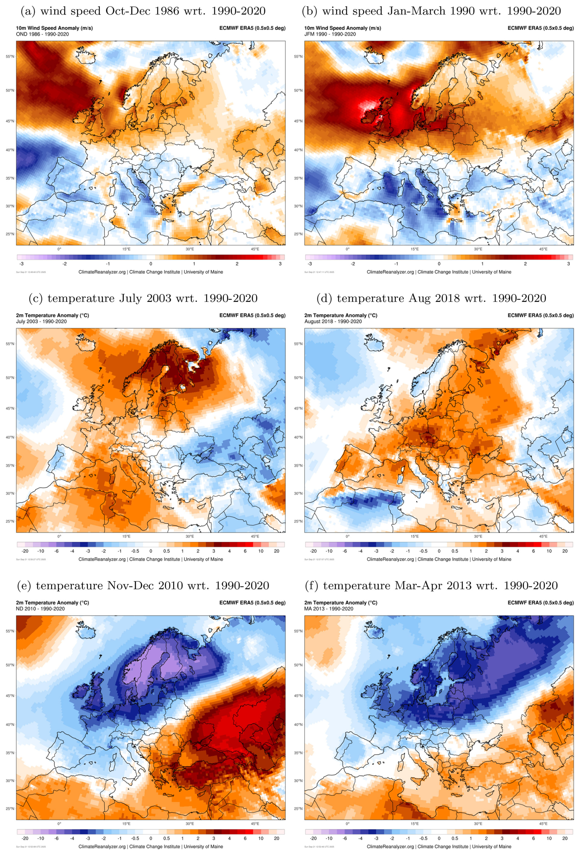
Figure C5 Examples of surface weather modulation during long-lasting weather regime life cycles. (a, b) Anomalies of 10 m wind speed in three-monthly periods as indicated in the subcaption. (c, d) Anomalies of 2 m temperature in a summer month, as indicated in the subcaption. (e, f) Anomalies of 2 m temperature in a two-months period, as indicated in the subcaption. The individual figures are produced with the tool (Climate Reanalyzer, 2025) provided by the Climate Change Institute of the University of Maine. ERA5 reanalysis data are used. The climatological period is the average of the indicated months and years 1990–2020.

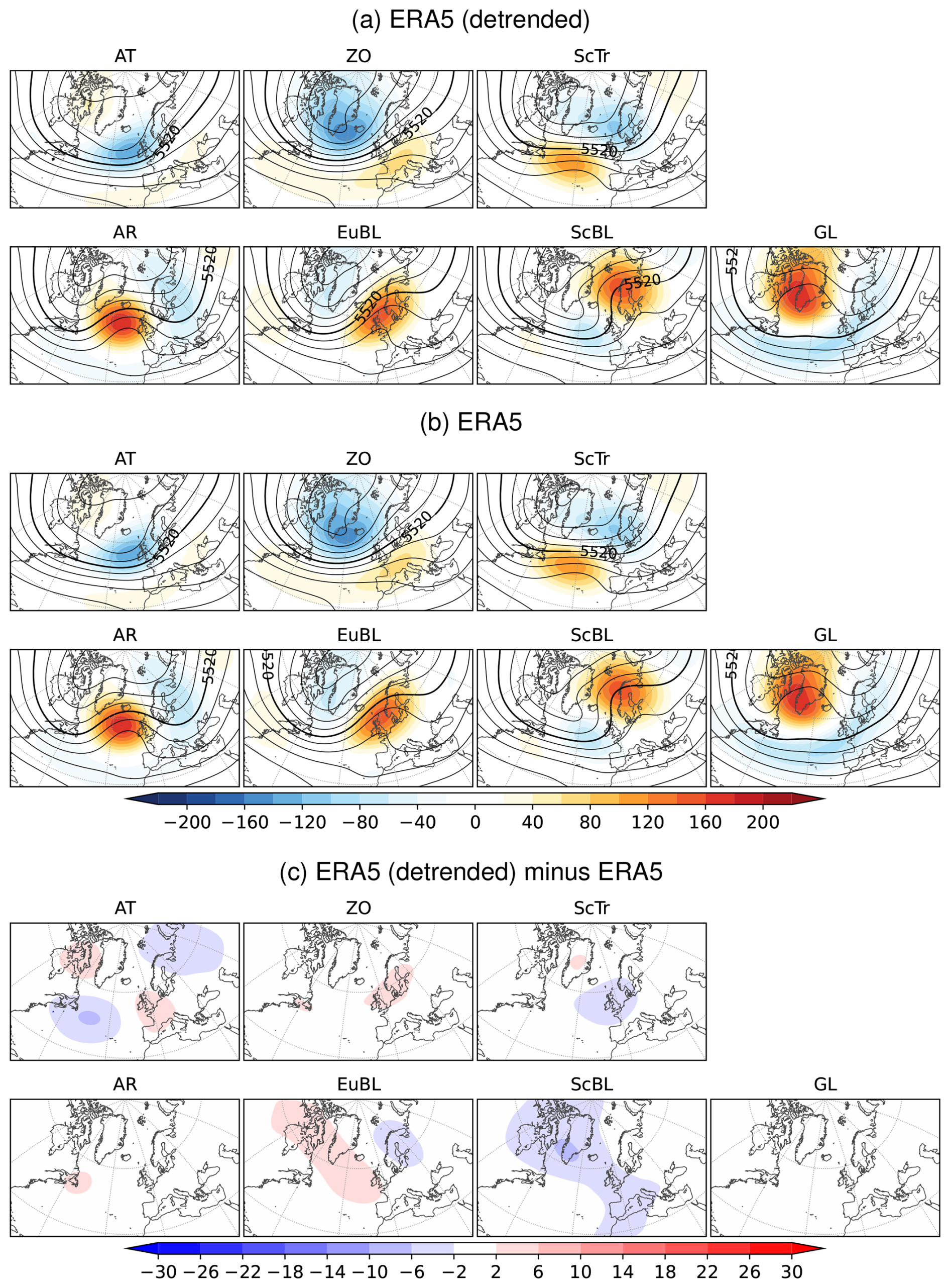
Figure C6 As in Fig. 2, cluster mean of low-pass filtered Z500 anomaly (shaded every 20 gpm) and absolute field (contours every 80 gpm, 5520 gpm in bold) based on the (a) ERA5 definition using detrended data, (b) original non-detrended ERA5 definition, and (c) the difference (in gpm) between the detrended and non-detrended definitions. The panel labels indicate the regime abbreviation. Both definitions are for the data period 1979–2019.

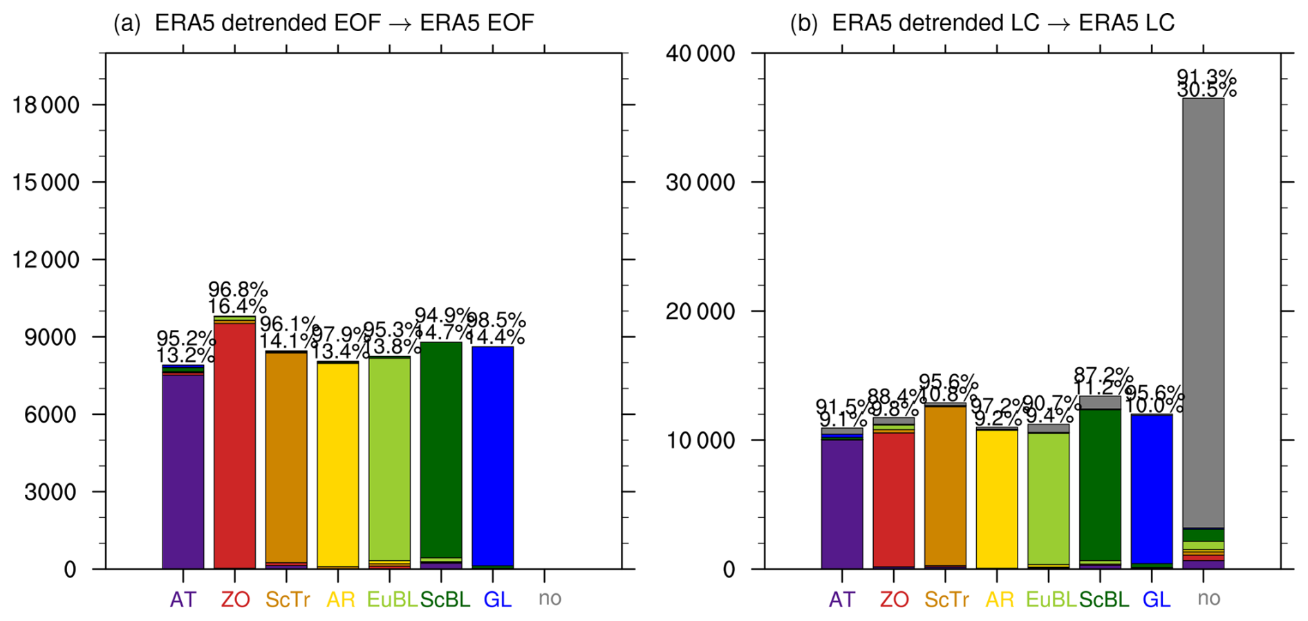
Figure C7 As in Fig. 5 frequency of the 7 regimes according to the raw EOF-cluster attribution and (b) frequency of the 7+1 weather regimes including the no regime class according to the life cycle attribution. Each bar shows the number of time steps (6-hourly in panel a for EOF attribution and 3-hourly in panel b for life cycle attribution) for the definition using detrended data on the x-axis. The lower numbers on top of each bar indicate the relative frequency of the regime. Coloured bar segments indicate to which regime these time steps are attributed in the original ERA5 definition using non-detrended data and the fraction of times sharing the same regime with the original ERA5 definition is indicated by the upper number. The data period covers 1979–2019.