the Creative Commons Attribution 4.0 License.
the Creative Commons Attribution 4.0 License.
 | 01 Feb 2022
Automated detection and classification of synoptic-scale fronts from atmospheric data grids
Stefan Niebler
Annette Miltenberger
Bertil Schmidt
Peter Spichtinger
Automatic determination of fronts from atmospheric data is an important task for weather prediction as well as for research of synoptic-scale phenomena. In this paper we introduce a deep neural network to detect and classify fronts from multi-level ERA5 reanalysis data. Model training and prediction is evaluated using two different regions covering Europe and North America with data from two weather services. We apply label deformation within our loss function, which removes the need for skeleton operations or other complicated post-processing steps as used in other work, to create the final output. We obtain good prediction scores with a critical success index higher than 66.9 % and an object detection rate of more than 77.3 %. Frontal climatologies of our network are highly correlated (greater than 77.2 %) to climatologies created from weather service data. Comparison with a well-established baseline method based on thermodynamic criteria shows a better performance of our network classification. Evaluated cross sections further show that the surface front data of the weather services as well as our network classification are physically plausible. Finally, we investigate the link between fronts and extreme precipitation events to showcase possible applications of the proposed method. This demonstrates the usefulness of our new method for scientific investigations.
- Article
(19136 KB) - Full-text XML
-
Supplement
(545 KB) - BibTeX
- EndNote


Atmospheric fronts are ubiquitous structural elements of extra-tropical weather. The term front refers to a narrow transition region between air masses of different density and/or temperature (see, e.g. Thomas and Schultz, 2019b). These air mass boundaries play an important role in understanding the dynamics of midlatitude weather and are usually related to clouds. Further fronts are often associated with significant weather, such as intense precipitation and high gust speeds (see, e.g. Catto and Dowdy, 2021; Catto et al., 2015; Martius et al., 2016). Hence, fronts in the sense of separating polar from more subtropical air masses play a vital part of the communication of weather to the public and the public perception of weather in general, although this aspect may have lost some attention due to the use of colourful apps. Frontal surfaces also exist on smaller scales, e.g. in the context of sea-breeze circulation or local circulation patterns in mountainous regions. Even tropical weather systems might indeed produce similar features of transition regions of different air masses, but due to other mechanisms than in extra-tropical weather systems. The focus here and in much of the literature is on larger-scale fronts that can extend over several hundred kilometres and are often associated with extra-tropical cyclones (Schemm et al., 2018). In addition, quasi-stationary fronts can also extend over a large distance, but they do not move strongly over time, e.g. the Mei-Yu front (e.g. Hu et al., 2021). These stationary fronts are also foci of significant surface weather. Unfortunately, there is no generally accepted front definition; see for example the discussion in Schemm et al. (2018) and Thomas and Schultz (2019a). Thus, the detection of fronts often relies on different measures, usually based on physical variables and including physical hypotheses or theories as detailed below. Additionally, it is still debated whether a front detection should be guided by determining surface fronts (such as on the analysis charts of weather services) or even more on the physical (horizontal and vertical) structure (see also the summary in Uccellini et al., 1992; Sanders, 1999).
Nevertheless, determining the position and propagation of surface fronts plays an important role in weather forecasting and, of course, in research on synoptic-scale phenomena. The traditional manual approach to front detection is based on the expertise of weather analysts at operational meteorological services, along some (mostly empirical) guidelines. With the advent of large, gridded datasets, e.g. reanalysis from different weather centres, such as ECMWF or NCEP, in the second half of the past century the drive for objective means to detect fronts automatically set in (see, e.g. Hewson and Titley, 2010). Currently used methods typically rely on detecting strong gradients in either temperature and humidity fields (e.g. by using equivalent potential temperature or wet-bulb temperature) or wind fields (Schemm et al., 2015). The former methodology goes back to the work by Renard and Clarke (1965) and is represented by Hewson (1998), who suggested an automatic method to detect fronts in fairly coarse datasets based on the so-called “thermal front parameters”, derived from thermodynamic variables. In these and subsequent studies this is often related to the second spatial derivative of the temperature, and one or more “masking parameters”, i.e. thresholds of thermal gradients along the front or in adjacent regions. This or conceptually similar methods have been used in numerous studies to determine the global or regional climatological distribution of fronts (e.g. Berry et al., 2011; Jenkner et al., 2010).
For the investigation of fronts on the Southern Hemisphere Simmonds et al. (2012) suggested an alternative approach that investigates the Eulerian time rate of change of wind direction and speed in the lower troposphere at a given location. A comparison of the two methods to identify fronts on a global climatological scale by Schemm et al. (2015) revealed some agreement between the fronts detected, but also regional difference and systematic biases in the detection of certain front types by both algorithms: for example, the “thermal” method more reliably detects warm fronts than the method based on lower tropospheric wind speed and direction. In addition, the orientation of detected fronts differs in general between the two methods. In consequence Schemm et al. (2015) also find differences in the global distribution of fronts and the amplitude of seasonal variations in front occurrence frequency.
While it is well known that different front detection methods provide different outputs (e.g. Schemm et al., 2015; Hope et al., 2014), an objective ground truth is difficult to find. Most studies developing or testing automatic detection schemes rely on manual analysis as the “gold standard” to test the accuracy and for tuning free parameters in the automatic detection schemes (e.g. Hewson, 1998; Berry et al., 2011; Bitsa et al., 2019). However, it should be noted that manual analysis is affected to a large degree by subjective decisions, and hence the focus, interest and expertise, of the person conducting the analysis. Shakina (2014) reports results from an inter-comparison study of different manual front analysis carried out independently in different divisions of the Russian meteorological service up until the 1990s. Comparing the different archives, agreement on the presence or absence of a front in any one box was found in 84.8 % of cases. However, if only the presence of fronts in any one grid box is considered, the agreement dropped to 23 % to 30 % depending on the type of front. Shakina (2014) further suggests that disagreement mainly arises from the detection and positioning of secondary or occluded fronts, which are typically associated with less marked changes in surface weather. It is likely that the differences between manual analysis by different forecasters in the meantime have not reduced, but they may potentially be reduced by strict guidelines for forecasters on the key decision features for positioning fronts.
Despite a non-negligible subjectivity of manual analysis, it still offers many advantages over automatic methods.
-
In contrast to most automatic detection methods, many different aspects, including temperature, wind, humidity fields, surface pressure, surface precipitation and wind, are taken into account.
-
Manual analysis does not rely strongly on the choice of (arbitrary) thresholds that are needed in most automatic front detection algorithms.
-
Experience of analysts can be taken into account, especially on regional scales (e.g. with complicated terrain such as in the Alps).
In order to address the over-reliance on specific variables, some recent studies have suggested methods that combine not only temperature and humidity data but also include information on the wind field (e.g. Ribeiro et al., 2016; Parfitt et al., 2017) or information on Eulerian changes in mean sea-level pressure (e.g. Foss et al., 2017). Nevertheless these extended algorithms that are so far mainly used in regional studies still rely on choosing appropriate thresholds for the magnitude of thermal gradients or changes in the wind direction and speed.
The necessity of manually designing metrics and selecting thresholds for automatic front detection can be at least partly overcome by employing statistical methods and machine learning approaches. The key idea with this approach is that based on manual analysis a complex statistical method retrieves as much consistent information on patterns, important variables and thresholds as is available in manual analyses and coinciding state of the atmosphere, e.g. from reanalysis datasets. Previous attempts at using machine learning approaches for front detection are discussed in more detail in the following section.
Bochenek et al. (2021) used a random forest to predict fronts over Europe using data from the German Weather Service (Deutscher Wetterdienst, DWD). Their results indicate that it is possible to detect fronts with this method; however it does not seem to be very robust, as the probability of object detection varies greatly between the shown samples.
Recently different groups have used artificial neural networks (ANNs) to predict frontal lines from atmospheric data. Biard and Kunkel (2019) used the MERRA-2 dataset to predict and classify fronts over the North American continent. Their network also classifies their predicted fronts using the four types: warm, cold and stationary fronts as well as occlusions. They used labels provided by the North American Weather Service (NWS).
Lagerquist et al. (2019) used the North American Regional Reanalysis (NARR) dataset (Mesinger et al., 2006) to predict synoptic cold and warm fronts over the North American continent also using the NWS labels. While the network of Biard and Kunkel (2019) creates an output on the input domain, the network of Lagerquist et al. (2019) predicts the probability for a single pixel and needs to be applied to each pixel consecutively. Both methods rely on post-processing steps like morphological thinning to create their final representation of frontal data. Additionally, both methods only use a 2D mask for each input variable, not making use of multiple pressure or height levels. Matsuoka et al. (2019) used a U-Net architecture (Ronneberger et al., 2015; Shelhamer et al., 2017) to predict stationary fronts located near Japan.
In this study we present a new method for automatic front detection based on machine learning using meteorological reanalysis as input data and trained with information on surface fronts provided by two different weather services (NWS and DWD). The overall aim is to investigate the degree to which machine learning approaches are able to replicate manual analysis on a case study and climatological scale and the degree to which the learned features are consistent with meteorological expectations on the physical properties characterizing a frontal surface. Our provided network uses the U-Net approach to predict and classify all four types of fronts and it does not require morphological post-processing. We evaluate our approach similar to Lagerquist et al. (2019) using an object-based evaluation method. Unlike the previous methods, we incorporate data from two different weather services, NWS and DWD, and also evaluate the two different regions covered by these datasets. We additionally compare our predicted fronts against the method developed by Schemm et al. (2015), using a thermal front parameter (TFP) as an example of a conventional automatic front detection method. We refer to it in the following as the “baseline method”. As input data we use the ERA5 reanalysis data (Hersbach et al., 2020) from the European Centre for Medium-Range Weather Forecasts (ECMWF) on a 0.25∘ grid at multiple pressure levels for each variable. This dataset exhibits a higher resolution than the NARR data (32 km grid) used by Lagerquist et al. (2019) and MERRA-2 data (1∘ grid) used by Biard and Kunkel (2019). In contrast to these studies, we also used multiple pressure levels to refine our results.
Although we are aware of the conceptual differences between determining surface fronts and the complex 3D structure of fronts, we use the surface maps as a ground truth, i.e. as a proxy for the complex structures called fronts. However, in the later evaluation it turns out that the detected surface fronts represent the expected physical properties of air mass boundaries in a meaningful way.
In Sect. 2 we describe our used network architecture, data and evaluation methods. In Sect. 3 we explain our evaluation methods and display our evaluation results on the training and test dataset. In addition we showcase applications in terms of determining the variation in physical properties across fronts (Sect. 3.2) and relating fronts to extreme precipitation events (Sect. 3.3). We close with a summary of the study and a short outlook for future improvements as well as further applications of the new method for scientific purposes.
For each spatial grid point our proposed algorithm predicts a probability distribution, describing how likely it is that the point belongs to each of our possible five classes: warm front, cold front, occlusion, stationary front or background. Our method predicts that probability from a four-dimensional input consisting of multiple channels located on a three-dimensional multilevel geospatial grid, which was flattened to a three-dimensional input by combining the atmospheric channel and level dimension. For this task we use a convolutional neural network (CNN) architecture to automatically learn atmospheric features that correspond to the existence of a weather front at spatial grid points. We use a supervised learning approach, in which we provide ground truth data of frontal data sampled from two different weather services (surface fronts). We adjust hidden parameters of the CNN in order to optimize a loss function measuring the quality of our weather front prediction. CNN architecture and training will be explained in further detail in this section. Our network was implemented, trained and tested using Pytorch 1.6 (Paszke et al., 2019). Parallel multi-GPU training was implemented using Pytorch's DistributedParallel package. The provided code was run using Python 3.8.2 and is freely available (see below).
2.1 Data
We will briefly describe which channels and grid points were used as training input from the ERA5 reanalysis data (Hersbach et al., 2020). Furthermore, we will describe the format of the corresponding label data of fronts obtained from NWS and DWD; in the case of the DWD label data, we additionally describe the pre-processing of the DWD data.
2.1.1 ERA5 reanalysis data
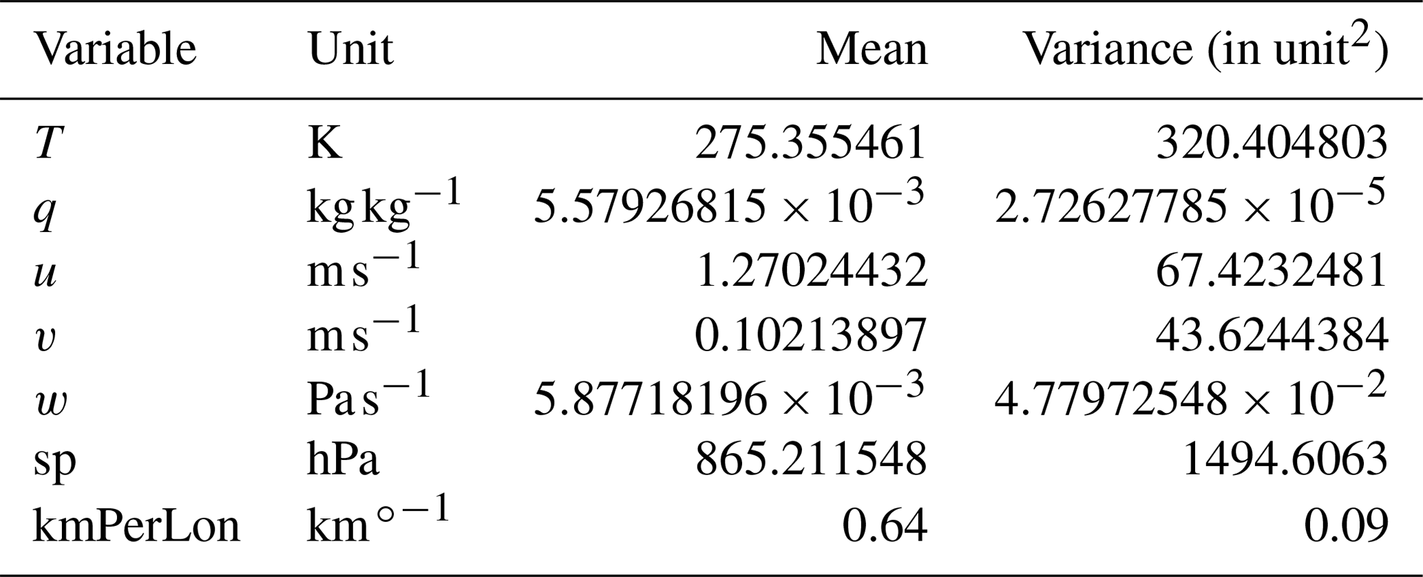
Our model input consists of a multichannel multilevel spatial grid provided by ECMWF's ERA5 reanalysis dataset. Each channel denotes a different atmospheric variable, while levels consist of a subset taken from the L137 vertical level definition (ECMWF, 2021). Data are represented on a spatial grid with a grid spacing of 0.25∘ in both latitudinal and longitudinal directions. Since we do not expect to obtain relevant information from high-altitude data, we decided to restrict ourselves to every fourth level within the inclusive interval [105,137], representing nine model levels between the surface and about 700 hPa. This range contains both the ground level information and the 850 hPa pressure level information, both of which are commonly used to detect fronts. Pressure values are defined as parameters of an affine transformation of the surface level pressure, which is why we manually added the surface pressure field to the data using the merge operation of the Climate Data Operators (CDO) (Schulzweida, 2019). This allows us to calculate the pressure at each grid point and level. We further only use five ERA5 multilevel variables as input for our network: temperature (T), specific humidity (q), zonal wind velocity (u, east–west), meridional wind velocity (v, north–south) and vertical velocity (w). In addition the surface pressure (sp) and longitudinal distance per pixel in kilometres relative to 27.772 km (kmPerLon) are considered. The distance between two pixels at a certain degree latitude is derived by assuming a spherical shape of the globe and is only used as a single level variable. Surface pressure on the other hand is used to estimate the pressure at each model level using the corresponding level parameter to create another multilevel network input. All resulting data are normalized with respect to a global mean and variance sampled from data of the year 2016. The resulting mean and variance values are listed in Table 1.
Table 1Mean and variance of the individual variables used for normalization of input data.
While ERA5 reanalysis data are available for the whole globe, the available ground truth labels only reside within the analysis region of their corresponding weather services. We therefore cannot use ERA5 data outside these regions. For this reason we decided to restrict our usage of ERA5 data to rectangular subgrids, each of which is completely within the analysis region of the respective weather service analysis.
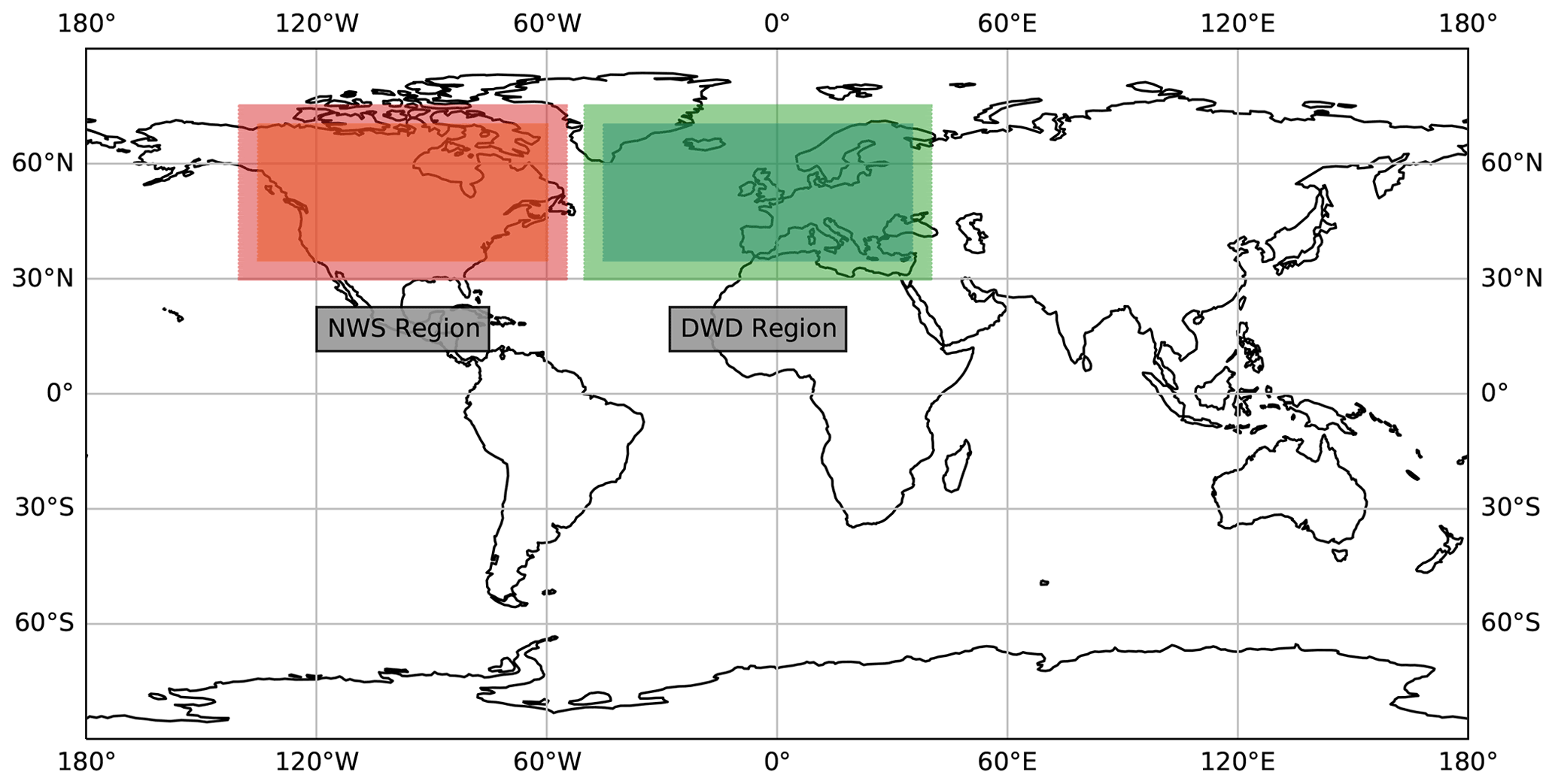
Figure 1Bounding boxes for the two regions used for training and evaluation against the weather service labels. The brighter area is used as input but is not used for evaluation.
The extent of these regions is described in Table 2 as DWDinput and NWSinput. Pixels at the border of our input may lose critical information to successfully identify a front due to the input crop. As a result detections on the outer 5∘ (20 pixels) of the input domain are not evaluated during training. While the network still outputs these pixels, they do not contain valid detections and should therefore be removed from the evaluation. As a result the effective output region is smaller than the input region, as indicated in Table 2. This is also shown in Fig. 1 as the difference in shade within each weather service region. Prior to evaluation we create detections for each sample using the global input data. Evaluations against the weather service labels are performed using the corresponding output regions. Comparisons against the baseline method use the same regions restricted to latitudes spanning N instead. The evaluation in Sect. 3.3 does not rely on the weather service data and is therefore evaluated within N and E. The restriction of the longitudes is caused by the smaller output regions, as explained in this section.
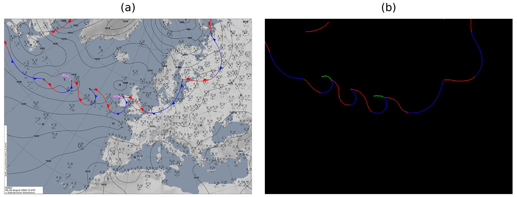
Figure 2Example of well-extracted fronts (b) from an image provided by the DWD (a) (source: DWD, 2021). In (b) blue and red lines correspond to cold and warm fronts as in the original image (a), and green lines correspond to occlusions which are pink in the input image. Note that stationary fronts are originally depicted as alternating warm and cold fronts. For this reason we cannot distinguish those from regular cold and warm fronts.
2.1.2 NWS front label data
For training on the North American continent, we use the HiRes Coded Surface Bulletins (csb) of the North American National Weather Service (National Weather Service, 2019). These data range from 2003 up to 2018 and were previously used by Biard and Kunkel (2019) and Lagerquist et al. (2019). Each front in a csb file consists of an identifier, describing the type of front, followed by a series of coordinate pairs on a 0.1∘ grid, defining a polyline of the front. We do not perform any pre-processing on these data. In accordance with our available data, we restricted the use of the latter to the years 2012 to 2017 using only snapshots in a 6 h interval to keep the amount of data balanced compared to the DWD data during training. The NWS dataset contains labels for the following front types: warm front, cold front, occlusion and stationary front.
2.1.3 DWD front label data
For training over Europe and the North Atlantic, we use label data extracted from the surface analysis maps of the Deutscher Wetterdienst (DWD) for the years 2015 to 2019. Unlike the coded surface bulletins, these maps are not provided as polylines but rather as PNG images of a region containing both the North Atlantic and western Europe (see Fig. 2a). Each of these images has a resolution of 4389×3114 pixels. To use the labels, we extract each individual front, by creating coordinate pairs, which describe the front as a polyline, similar to a csb. Within an image different types of fronts are colour coded, which allows us to easily separate them from the background. Our algorithm first filters all fronts of a specific type by filtering all pixels of the corresponding colour. In a second step we erase all additional symbols on each line. This includes symbolic identifiers like half circles and triangles, indicating the propagation direction of a front, as we do not need this information. Also, otherwise, these symbols could create false positive coordinate points in the label data. Subsequently, latitude and longitude coordinate pairs along each line are extracted in order to describe each front in terms of a polyline. In Fig. 2b we show an example of a processed image file, redrawn onto the same projection as the input image. Blue and red lines in both panels correspond to cold and warm fronts respectively, while green lines correspond to occlusions, which are pink in the left panel.
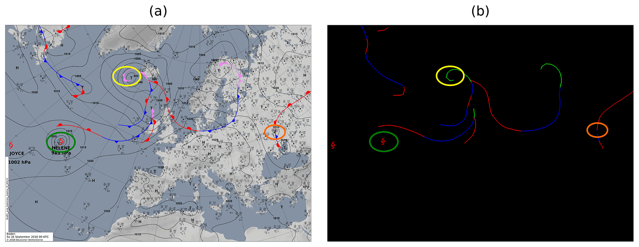
Figure 3Example of badly extracted fronts (b) from an image provided by the DWD (a) (source: DWD, 2021). The green circle shows an object that is not a front but has the same colour coding that is wrongly extracted as a front. The orange circle is an unrelated symbol drawn over the front. The front could not be extracted completely. The yellow circle is a frontal symbol placed in an area with high curvature. The curvature is not extracted exactly, as the symbol is removed during the procedure, and the loose ends are connected with a straight line.
In certain cases our method fails to correctly extract the frontal lines. These cases lead to gaps within a front, wrongly extracted objects or wrongly connected fronts. Gaps originate from two factors. One is that another object is drawn on top of a frontal line, effectively splitting the front into two parts. The other is an aggregation of multiple front symbols on a short segment. As our method removes sections where a symbol is placed before reconnecting the remaining points, crowded placement of these symbols may make the remaining part of the front too short to be considered relevant and as such will be omitted. Wrongly extracted objects occur mostly due to tropical storm symbols that are depicted in the same colour as a warm front. As such our extraction method wrongly extracts these objects as well. Finally, errors can occur when we try to sort the extracted coordinate pairs of a single front. In some cases the sorting method may end up stuck in a local minimum, resulting in a wrong order of points. An example of such a faulty extracted image is shown in Fig. 3. However, these are relatively rare and only account for a small portion of fronts within a sample, and many are going to be masked by the lower resolution of ERA5, which is why we ultimately decided to ignore these cases for this work.
We can extract information for the following front types: warm front, cold front and occlusion. Since stationary fronts are indicated by alternating warm and cold fronts, we cannot extract this information from the images as obtained from DWD; this would interfere with the classification of warm and cold fronts.

Figure 4U-Net architecture used in this paper. The first convolution of the input data uses a 1×1 sized kernel instead of 5×5. Decode and encode blocks are explained in the boxes at the bottom of the image. Each decode and encode block consists of three sequential blocks: convolution, ReLU and BN. U×V describes the image size per channel. Cin and Cout describe the number of channels of the input and output of an encode or decode block. The copy operation simply copies the blue box at the start of the arrow into the white box at the end. The white and blue boxes then describe the concatenation of the output from the copy and upsample operations. The number at the left-hand side of each block denotes the spatial input dimension. The shown sizes are those used during training; however the initial spatial dimension can be chosen freely as long as it is divisible by 8. At each red (green) arrow the dimension is divided (multiplied) by 2. The number on top of each block denotes the number of channels for each block and must not be changed.
2.2 Network design and training
2.2.1 Network architecture
Neural networks are a machine learning technique where a network consisting of several layers is used to extract feature representations of an input at different levels. Each layer transforms its input into an output map, the layer's feature map. These feature maps can then be used as an input for consecutive layers, which enables the network to learn more detailed features within the data. In a convolutional neural network (CNN) the most common transformation function is a convolution of the input image with a convolution mask where each entry is a trainable, latent parameter of the network. During training these parameters are adjusted to optimize a loss function, which measures the quality of the output of the network. In our case we use a U-Net architecture originally introduced by Ronneberger et al. (2015) for biomedical segmentation. The proposed architecture consists of several consecutive blocks that gradually extract features from the data and reduce the spatial dimension of the input data to extract features on multiple scales (Fig. 4). These blocks are followed by a number of expansive blocks which gradually increase the resolution up to the original scale. Additionally at each resolution scale a so-called skip connection allows the final feature map of an encoding block to directly serve as additional input to the corresponding decoding block, displayed as grey arrows in Fig. 4. These skips improve the networks' ability to localize the features, as the upsampled features only hold coarse localization information. In our network we use convolutional layers as explained before. Additionally we use rectified linear unit (ReLU), batch normalization, pooling, upsampling and 2D-dropout layers, whose functionality we will briefly explain. The dropout chance at each 2D-dropout layer is set to 0.2.
-
ReLU layers are used to introduce non-linearity into the network. They transform each input x as .
-
Batch normalization layers normalize the batched input to a mean of 0 and variance of 1. They can have additional learnable affine parameters.
-
Pooling layers transform several input grid points to a single output grid point. Common operations are averagePooling or maxPooling where the grid points are combined calculating the average or maximum of the input respectively. This operation is used to reduce the resolution of the feature map.
-
Upsample layers are a simple upsampling of a grid point to increase the resolution of the feature map.
-
2D-Dropout layers randomly set all values in a channel to 0 to reduce overfitting.
A sketch of the used architecture is shown in Fig. 4. We use Pytorch's DistributedParallel package to enable training on multiple GPUs in parallel. Training is performed on a single node, with each GPU acting on a fixed shard of the available data.
Table 2The input and output regions for the respective weather service analysis dataset used during training and the global input region. Levels are only used for network input. The output regions are also used during evaluation against the weather service labels. Every fourth vertical level between levels 105 and 137 is chosen to reduce the amount of input data, also in terms of redundant information.

2.2.2 Dataset augmentation
In each epoch and for each timestamp, we randomly select one of the available weather service labels for the given timestamp. Depending on which weather service was chosen, we crop a 128×256 pixel sub-grid residing within the corresponding weather services' input region (see Table 2) from the ERA5 data. We use this smaller crop instead of the complete region to increase the number of training samples, reduce the memory footprint on the GPU during training and ensure that all input dimensions are multiples of 8. The extracted label data are also cropped by removing each vertex, where neither the vertex itself nor a neighbouring vertex is located within the extent of the ERA5 crop. To further increase sample count via data augmentation, we also perform random horizontal and vertical flips on the data. It is important to note that, whenever data are horizontally (vertically) flipped, the sign of the input variable v (u) has to be flipped as well, as these variables describe a vector field rather than a stationary value. Flipping of the data might also lead to a better representation of fronts in the Southern Hemisphere, which are “mirrored” at the Equator (see Video supplement Niebler, 2021c).
2.2.3 Training
Our model is trained using stochastic gradient descent with Nesterov momentum of 0.9 to minimize the loss function. The initial learning rate is set to 0.005 ⋅ #Ranks, where #Ranks corresponds to the number of processes used for the parallel training. We train the network for several epochs. Within each epoch the algorithm randomly trains on a permutation of the complete training dataset. Every 10 epochs we measure the training loss. If the test loss does not improve for 10 test phases we divide the learning rate by 10 up to a minimum of 10−7 and reset the count, if the learning rate was changed. If the test loss does not improve for 20 test phases (200 epochs) and we cannot reduce the learning rate anymore we stop training. Additionally we set a maximum of 10 000 training epochs or 3 d time as stopping criteria. At each test step, we save a snapshot of the network if the test loss is better than the currently best test loss. Our final network is the resulting network which yielded the lowest test error.
2.2.4 Label extraction
As described by Lagerquist et al. (2019), the frontal polylines are subject to two non-negligible causes of bias: inter- and intra-meteorologist. The first bias describes the effect of two meteorologists disagreeing on the exact location of a front, the occurrence of a front at all or which exact shape the frontal curve follows. The second bias describes the effect of the same meteorologist being biased on the placement of the frontal line due to fronts placed at previous analysis times by the same person.
The transformation of these curves into polylines and the application onto a different resolution is subject to creating additional label displacements. While these problems are present in most human-labelled data, it is more peculiar in this specific case because the ideal polyline should have a width of only a single pixel. As a result each ever-so-slight displacement introduces a large per pixel disparity between two fronts, as the intersection of the sets of pixels that describe these fronts ends up being close to nonexistent. This has at least two negative effects. First, the gradient information is really sparse, as a close prediction will be considered a false positive just as a far off prediction, as can be seen in the example of Fig. 5a. Further translating the green line to the right will barely affect the count of intersecting pixels with the red line, even though one would expect the detection to become worse the further it moves from the label. Secondly, the previously mentioned label offset due to personal bias may lead to the case that a labelled front is not located exactly at the physical frontal position, essentially creating a false label with wrong underlying atmospheric properties. Due to the low intersection count, a correctly placed detection will now score badly.
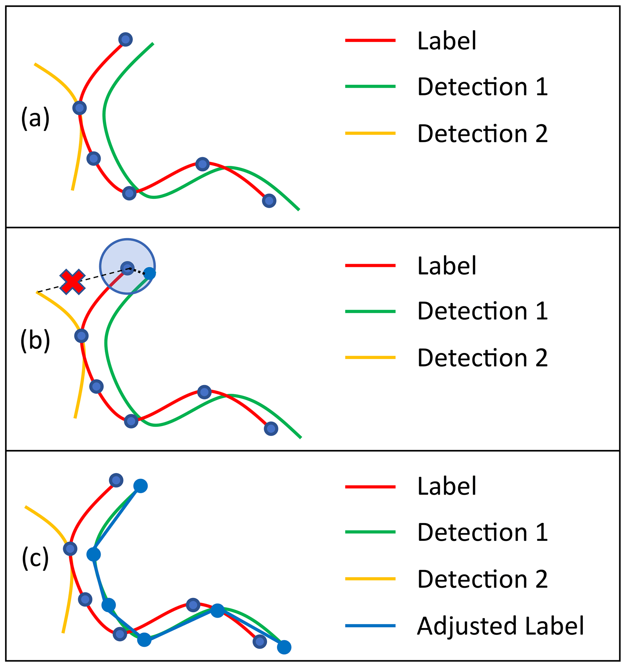
Figure 5Sketch of our label adjustment method. (a) Initial weather service label with polyline vertices (blue dots) and two possible detections. Detection 1 initially scores lower than Detection 2 due to a lower intersection with Label. (b) Display of how a vertex of Label might be adjusted within a search radius for Detection 1. The possibly optimal position for the vertex regarding Detection 2 is not within the search radius of the vertex. Deformation will therefore not be able to create a good intersection of the upper part of Detection 2 and Label. A similar situation occurs for the three vertices at the bottom right of Label. (c) Possible resulting Adjusted Label after each vertex was adjusted. The Label was deformed onto Detection 1 as it creates the best matching score. Detection 2 is too far from several vertices of Label and cannot score a similar matching score with any deformation of Label. As a result, Detection 1 now scores higher than Detection 2.
One way to handle this might be to widen the extracted front labels. While this approach introduces further false positive labels, slight translations in the detection are less penalized as they are more likely to be covered due to the larger width of the labelled data. Additionally the network is inclined to also detect wider frontal lines, making it even easier to create intersections. In the same way the effect of positional bias of the label placement is also reduced as the widened label is more likely to cover the physically correct location, if a small translational bias exists. However, this bias is not completely negated. From our studies and the results of previous studies (e.g. Matsuoka et al., 2019; Lagerquist et al., 2019; Biard and Kunkel, 2019) it seems apparent that a deep learning architecture learns that a bias in label placement exists and as a result tends to predict enlarged lines, trying to cover the uncertainty caused by the bias. Using enlarged labels further enhances this effect, leading to even larger line width, which in return leads to a low spatial accuracy of the detections. To regain positional accuracy, previous work used a morphological post-processing step to extract thin lines from wider network predictions.
In this work we use a different approach, as illustrated in Fig. 5b and c, to counteract this initial loss of positional accuracy. Instead of widening the label, we deform the given polylines prior to evaluation, by translating the vertices within a restricted search radius (panel b). All possible deformations are considered and evaluated according to a matching function, and the highest scoring deformation is then used for evaluation (Fig. 5c). This approach encourages the network to predict fronts with a high spatial certainty, as the labels themselves remain thin, while the deformation models the positional bias.
A polyline j consists of a series vj of vertices vj,i, where each vj,i describes the coordinate pair of the vertex as it is extracted from the weather service label. Additionally each deformed polyline contains a series of translations trj, consisting of a translation vector , which describes the translation of vj,i within the polyline j. A segment of the deformed polyline j is the edge ej,i connecting and . We calculate the matching score of a segment as follows:
-
calculate the positions of pixels of the line connecting and ,
-
sum the values of all pixels in the network output that are on this line,
-
weight the sum by , and
-
reduce the result by the number of pixels in the line connecting vj,i and .
The matching score of a polyline is considered the sum of the matching scores of each line segment of the deformed polyline.
The third step models the assumption that the provided labels are generally placed correctly and that strong deformations are less likely. Therefore a low deformation is preferred to a strong deformation if the intersection with the network output is the same. This matching procedure operates ignorant of the classification results and only takes the presence or absence of any type of front at a given pixel into account. We restricted ourselves to deformations where with k=3, keeping the deformation radius small to only counteract the positional bias of the label, which we expect to be small. Additionally we chose σ=k. We do not change classification information of the labels during the procedure. Thus each front is extracted as the class provided by the weather service. This matching procedure was implemented using C++ and Pybind11 v2.6.0 (Jakob et al., 2017).
This method comes at the risk that instead of predicting the position of the front the network may end up detecting a systematic displacement of the front within the range of the grid. We believe this could happen for two possible reasons: (i) the label bias exhibits a systematic displacement itself, and (ii) k is chosen too large. In the first case the error lies within the labels, and it is generally questionable whether or not these labels are suitable for training at all. The parameter k controls at which distance from the labelled front the detection may still be considered correct. With increasing k the incentive to place the detection close to the provided label reduces, diminishing the spatial accuracy of the predictions. Therefore we have chosen k=3, allowing each vertex to displace itself up to three pixels in each direction, limiting the scope of movement to a sensible range.
As an example, Fig. 5 shows how this algorithm can help to solve the problem of a correct detection being penalized by a biased label. We assume that the green line (Detection 1) is a correct detection with appropriate underlying atmospheric properties, while the yellow line (Detection 2) is an artefact caused by unfinished training of the network. Additionally the red line was drawn biased and is therefore not located at the appropriate position, regarding the underlying atmospheric features. In Fig. 5a the correct prediction has very few pixels intersecting with the label, similar to the wrong prediction. Not performing any deformation would wrongly count several pixels of the green detection as false positives, while only resulting in a similarly low number of pixels considered true positive similar to the yellow detection. However when using the deformation algorithm most pixels of the green detection correctly count as true positives, while the yellow detection is correctly classified as false positive. A deformation towards Detection 2 does not occur in this example, as the yellow line is out of range for most vertices. Most segments will therefore not intersect with the yellow line, leading to generally lower matching scores than the displayed blue line. The latter further displays the importance of the choice of k for preventing the label from deforming onto a wrong detection.
2.2.5 Loss functions
During training we extract the label lines as described in Sect. 2.2.4. As a loss function we decided to use a loss based on intersection over union (IoU), which we evaluate for each output channel individually, before combining them by a weighted average. This loss function inherently circumvents the problem that in each channel most of our output belongs to the background as it does not contain a front. While the original formulation of IoU is used for sets and therefore a strictly binary labelling, we used an adjusted version that works with floating point probabilities. This loss function is also used by Matsuoka et al. (2019). However, they only evaluate it on a single output channel. The definition of loss for a single output channel is given by the following equation:
Here L denotes the loss function, x is the extracted label image and p is the prediction of our network. pi and xi are the ith pixel of either p or x. We subtract the loss function from 1, as we will minimize our loss function during training, as the IoU normally increases the better the prediction becomes. L(p,0) always evaluates to 1 regardless of p, which means we do not obtain much information from such a label. When combining our network's output channels, we try to adjust for this problem. We define a variant of L, denoted as L0, that simply omits evaluation for all L0(p,0) values by setting the result to 0. In all other cases L0=L. These omitted cases therefore will not influence the training gradient. As our network generates a multichannel output, we calculate a loss for each channel individually and combine the results. The first output channel corresponds to the background label, which corresponds to the absence of fronts. We invert this output, by subtracting it from 1, to get a value describing the presence of fronts. As a result we obtain five output channels describing fronts (front, warm front, cold front, occlusion, stationary front) denoted as . Additionally in each batch b we have batchsize samples bn, and for each bn we have a detection and a label . The respective data in the channel k are then denoted as and . For each bn we calculate . For the classification channels k>0, we calculate instead and denote these results as correspondingly. By doing so, we may omit some samples where no label is present within the respective channels. To compensate, we define a weight for k>0, where nzb,k is the number of samples in b where there is any label in channel k. This weight is used to balance the potentially different counts of labels for the individual channels. The resulting loss for one bn∈b is calculated according to
The values 0.2 and 0.8 are chosen to formulate a weighted average over all channels. In the case of , we set . In this case channel k will not be evaluated at all within the current batch. The loss for the complete batch can then be calculated as the mean of all values within the batch b:
2.3 Baseline method
We compare our results against a baseline method developed and used at ETH Zurich. The method introduced by Jenkner et al. (2010) and later modified by Schemm et al. (2015) uses thermal gradients and other information to predict fronts. While the method was originally designed to work on a 1∘ resolution grid, we adjusted the hyper-parameters of the method to allow it to run on a 0.5∘ grid1. In the baseline method, i.e. that designed for the ERA-Interim dataset with a grid spacing of 1∘, a minimum equivalent potential temperature gradient of , a minimum advection velocity of 3 m s−1 and a minimum front length of 500 km are used. We decided to keep these physical values identical to the original algorithm to retain similar physical properties of the front. However, we have altered parameters used for the a priori smoothing of the equivalent potential temperature gradient field (number of filter applications as described in Jenkner et al., 2010, increased from five to seven), the smoothing of frontal lines (smoothing parameter changed from 5 to 15) and the minimum size of front objects in number of grid points (increased from 15 to 20). The largest impact comes from adjusting the smoothing of the equivalent potential temperature gradient field. Using these altered settings, the number of fronts detected in the northern and southern extra-tropics increases by about 30 %, but the spatial distribution of fronts is very similar to the original ERA-Interim dataset with some exceptions in the vicinity of steep terrain (not shown). Our network works on a 0.25∘ resolution grid and outputs on the same domain. Therefore, when comparing against the baseline method, we resample the network output to a 0.5∘ resolution using a 2D maximum pooling operation. The authors of the baseline method mention that the provided baseline should only be applied to the midlatitudes. When comparing against the baseline, we therefore restrict ourselves to the midlatitudes of the Northern Hemisphere for a fair evaluation.
2.4 Evaluation methods
We will briefly explain how the data are processed for the evaluation and how the critical success index (CSI) is calculated.
2.4.1 Trained models and dataset distribution
We distribute our data into a test (year 2016) and a validation (year 2017) dataset and create three training datasets as described in Tab. 3. We train a total of three models, one for each training set. The models trained using training NWS (training DWD) are additionally restricted to only use label data from the NWS (DWD) during training. Each model is trained using six GPUs on a single node of the Mogon II cluster of the Johannes Gutenberg University. Each node contains six Nvidia GeForce GTX 1080 Ti GPUs and an Intel Xeon CPU E5-2650 v4 with 24 cores and hyperthreading. Data were staged in prior to training to enable reading from a local SSD rather than the parallel file system. The models trained using training NWS and training DWD are only used in Sect. 3.1.1 with results presented in Tables 4 and 5 as well as in Tables S1 and S2 in the Supplement. In all other cases the model using training both is applied.
Table 3Distribution of our data into training, validation and test datasets. For each dataset the covered time frame and number of labels are shown. All models use the same validation and test data.
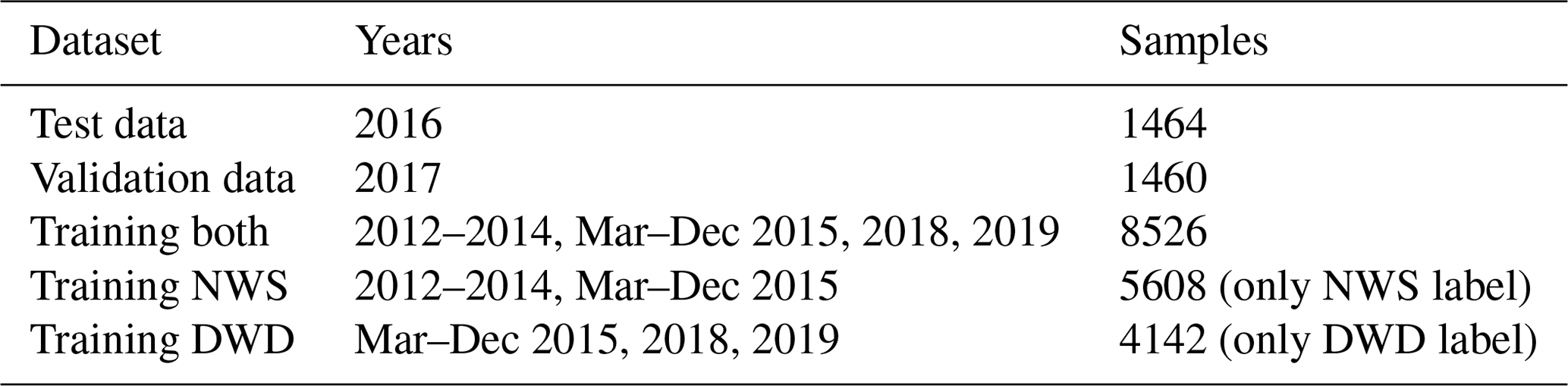
Table 4CSI, POD and SR values for D=250 km evaluated on DWD data for 2016. Warm fronts tend to be detected worse than the other classes while cold fronts are generally well detected. Stationary fronts are not available for DWD labels and are therefore not listed. Evaluation regions contain latitudes within ( N].
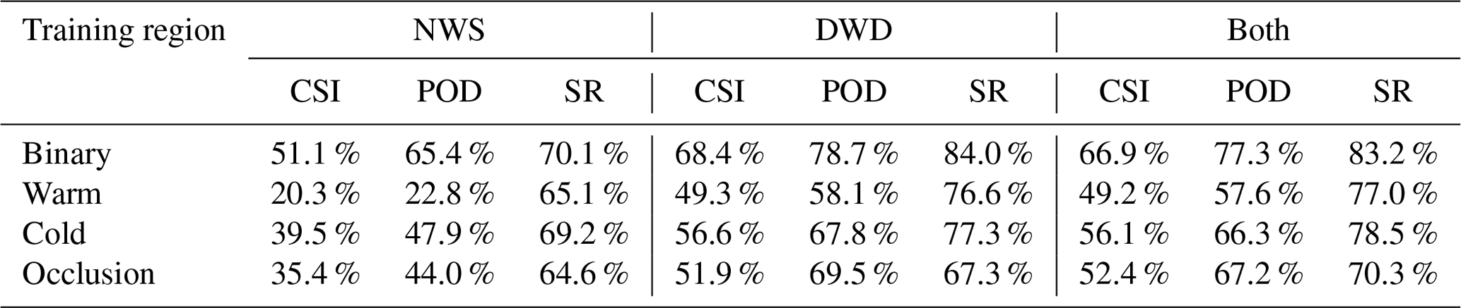
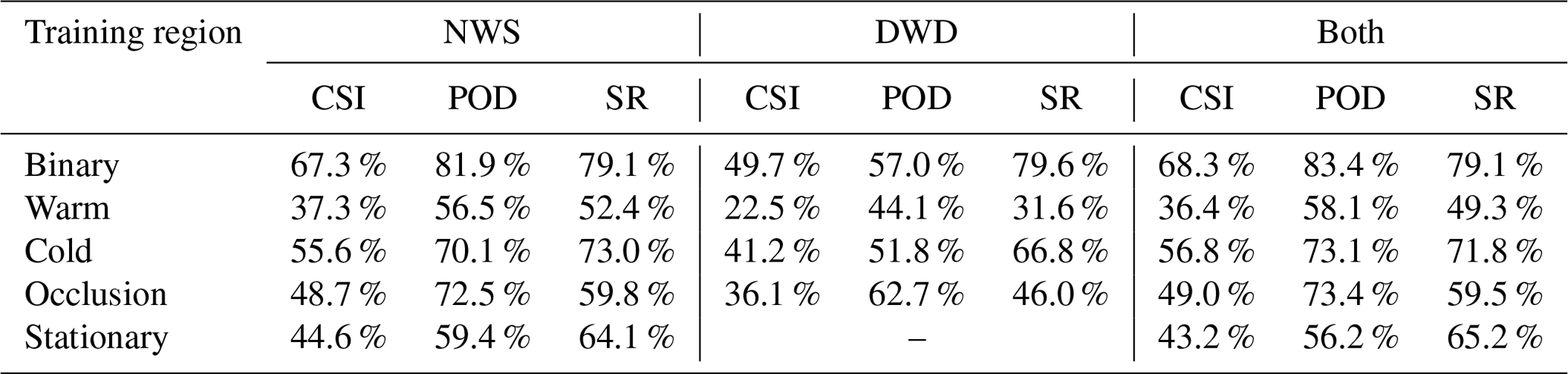
Table 5CSI, POD and SR values for D=250 km evaluated on the NWS data 2016. Warm fronts tend to be detected worse than the other classes while cold fronts are generally well detected. The network trained purely on DWD data could not learn stationary fronts, as they are not included in the training data, and stationary fronts are therefore not listed. Evaluation regions contain latitudes within (] N.
2.4.2 Test data processing
For the evaluation we process each input file in the test dataset as follows.
-
Apply the respective model to the global input region of the current sample.
-
Apply a softmax activation function to the raw network output to generate a probability mask for the sample.
-
Create a binary mask by setting each entry in the probability mask to 1 if it is greater than 0.45, otherwise to 0.
-
Use one iteration of eight-connected binary dilation and calculate all different connected components. Each connected component is considered an individual front.
-
Filter the labelled image with the undilated binary mask to remove the dilation effect.
-
Remove all fronts that consist of fewer than two pixels.
-
Write the binary mask to disc.
During evaluation we then load the corresponding binary mask from disc and crop it to a sub-region when necessary. Results of the baseline method and the weather service labels are already provided in binary format.
2.4.3 Front to object conversion
Prior to evaluation the generated binary masks of our network output are transformed into front objects in two steps.
-
Use one iteration of eight-connected binary dilation and calculate all different connected components. Each connected component is considered an individual front.
-
Filter the labelled image with the undilated binary mask to remove the dilation effect.
The same transformation is applied to the provided weather service fronts. Note that some provided weather service fronts are separate lines in the label file but end up as a single longer front due to being connected due to the coarser grid used in our analysis.
2.4.4 Front object matching
A predicted front Fp is considered to be matched to the weather service label if the median distance of each pixel of Fp to the nearest labelled pixel of the same class in the weather services' label image is less than a detection radius of D. The same is applied vice versa for the weather service fronts compared against the network output. Each class of front can only be matched to pixels of the same class; however each frontal object is matched against the whole set of pixels of the same class, rather than just a single other object.
For the evaluation we define two distinct regions, namely (i) the evaluation region, which is the region out of which we take the fronts we want to match against any other fronts, and (ii) the comparison region, which is the region in which the algorithm checks for possible matches for the fronts within the evaluation region. In our evaluation the comparison region is the same as the evaluation region with an additional extension of 10∘ in each direction. The advantage of looking for matches within this comparison region instead of the evaluation region is to reduce false results caused by the crop of the evaluation region: for example, fronts at the edge of the evaluation region may be split into multiple fronts due to the crop skewing the count of individual fronts. Alternatively a front located at the edge of the evaluation region may be counted as unmatched because the possible match was cropped out. Using the comparison region we will resolve most of these cases. A sketch of this procedure is shown in Fig. S1. Note that using this larger region for the matching purposes does not add any fronts to the evaluation, nor does it affect the matching radius D. This change only allows each front to better use its search radius D to find possible matches unaffected by input crop.
2.4.5 Critical success index calculation
We evaluate the detection quality of our network and the baseline method by calculating the critical success index (CSI) similar to Lagerquist et al. (2019). As ground truth the provided weather service labels of surface fronts are used. We define nMWS as the count of fronts provided by a weather service that could be matched against the prediction, while nWS is the count of all provided fronts. Similarly, nMD describes the count of all detected fronts that could be matched against the weather service fronts, while nD describes the total count of detected fronts. With these values we can then calculate the critical success index (CSI), probability of object detection (POD) and success rate (SR) as described in Eqs. (4)–(6) respectively.
As mentioned by Lagerquist et al. (2019) these measurements are also applied in other scenarios, like the verification of tornado warnings by the NWS (Brooks, 2004). The SR describes the probability that a predicted front corresponds to an actual front from the labelled dataset, while the POD describes the probability that an actual front is detected by the network. SR and POD could easily be maximized at the cost of the other, by either not predicting anything or classifying each pixel as a front instead. The CSI serves as a measurement that penalizes such degenerate optimizations as it maximizes only when both values yield good results. Generally speaking, a high CSI score is preferable. Whether it is more important to have a high POD or SR depends on the task at hand and whether it is more important that the detection is more sensitive or more accurate.
In this section we first evaluate the CSI of our network detections against the weather service data and compare the detections from the network to those from the baseline method (Sect. 3.1.1). We additionally create climatologies for both automatic methods and calculate the Pearson correlation against climatologies created from the weather service data (Sect. 3.1.3). Secondly, we present further results of our networks' output where we look into physical quantities across the frontal surface to infer physical plausibility of our network's detections. Finally, we evaluate the relation of fronts to extreme precipitation events to highlight a possible scientific application scenario for the presented method (Sect. 3.3).
3.1 Performance evaluation and comparison against baseline
3.1.1 Front detection quality
In Fig. 6 we provide an image showing an example of the networks' output compared to the label of the corresponding weather service. The image shows that the network tends to create thin fronts, as desired. The detections also appear to have a generally smoother shape compared to the weather service labels. The general shape of the fronts appears plausible, even though there are disagreements between the detections and labels regarding both the shape and class of fronts. For a better impression of the networks' output, we also provide a Video supplement showing the network output on a global scale (Niebler, 2021c). Further details are provided in Sect. S4.
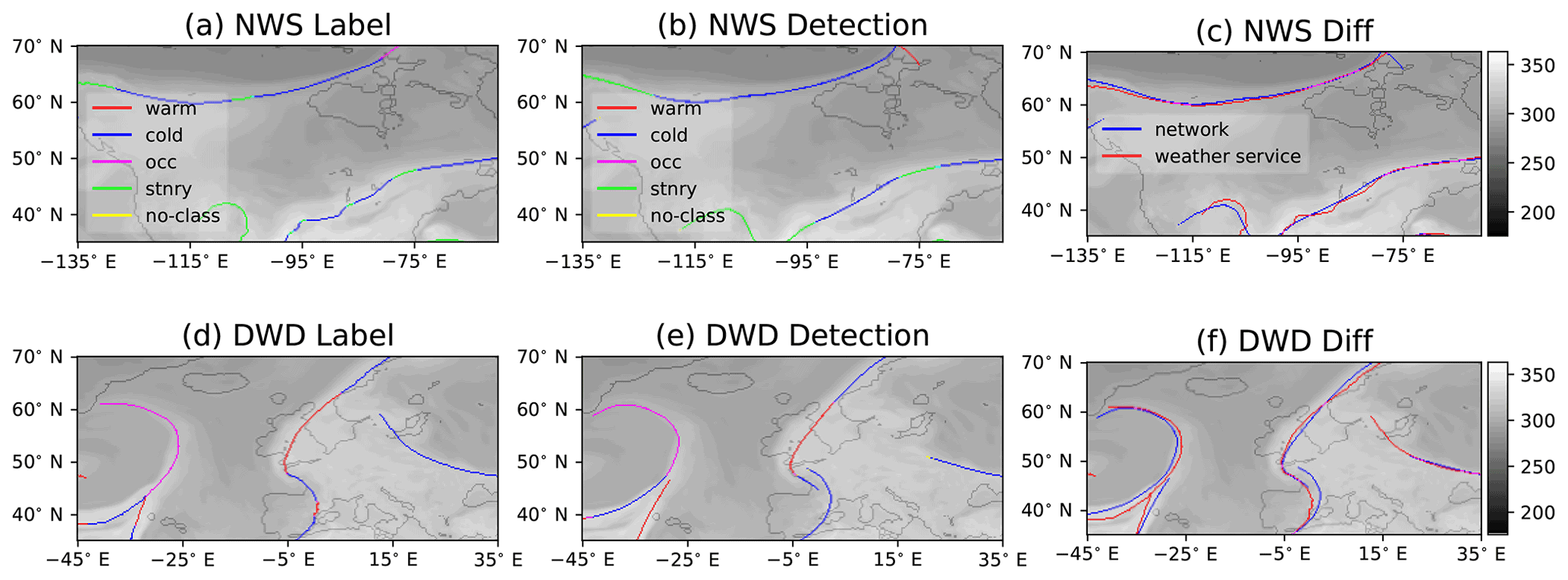
Figure 6Fronts from provided labels of the NWS (a) and DWD (d) as well as the corresponding network-generated outputs (b, e) displayed on top of equivalent potential temperature. Colours indicate the frontal type, whereas unclassified fronts are displayed in yellow. The labels are the same for both rows. The difference images (c, NWS) (f, DWD) show a direct comparison of frontal placement by the weather service (red) and the network (blue) ignoring classification. All displayed examples are on 14 September 2016 at 00:00:00 UTC.
To quantify the quality of our predictions, we evaluate the CSI, POD and SR for a matching radius of D=250 km on our test dataset. The results are listed in Tables 4 and 5 for the binary task, which only considers the classes front and no-front as well as the individual scores for each of the four frontal classes. As evaluation region we use the corresponding weather services' output region as defined in Table 2.
The scores show that the network excels at the pure front detection task with CSI scores of 66.9 % (DWD) or 68.3 % (NWS). At the same time the network evaluates with a POD and SR exceeding 77.3 %. POD tends to be higher than SR for the NWS data, while on the DWD data SR tends to be higher than POD. Considering individual front classes, the classification scores are overall lower, with a class CSI ranging between 36.4 % and 56.8 %. Across all tests, warm and stationary fronts appear to be harder to classify for the network than cold fronts or occlusions. This effect is more pronounced on the NWS dataset. A possible explanation is the lack of a clear distinction of these two front classes from the DWD data, which in return leads to more false classifications due to the ambiguity. We can further see that training on a single region does not provide a good generalization onto the other region, which is expressed by lower CSI scores when training on only the DWD (NWS) data and evaluating on the respective other region, i.e. NWS (DWD) data. At the same time training on both regions yields comparable scores as the networks trained on a single region. This clearly shows that using the network trained on both regions is preferable. We will therefore continue our evaluation with only this model. The difference between the regions may be originating in different synoptic structures of cyclones and their associated fronts over the North American continent and over the North Atlantic. This implies that the inclusion of further datasets, for example datasets used by Matsuoka et al. (2019) or generally data of the Southern Hemisphere, may improve the network performance even further. This would also be interesting with regard to a thorough evaluation of the network performance on the Southern Hemisphere. We want to point out here that the inclusion of additional training data of similar structure to the used NWS/DWD data can be carried out easily; the method is designed to be very flexible.
We also evaluated results where each object can only be matched against a single object of the corresponding class instead of the whole set. The resulting scores are listed in Tables S1 and S2. We observe a drop in POD from 77.3 (83.4) to 70.8 (76.9) when evaluating on DWD (NWS) data, while SR barely changes. This indicates that our network tends to not fully cover long frontal regions with a single front but rather multiple smaller, disjointed fronts. Each of these can still be matched with the long front, but the long front cannot be matched with any one of them due to their insufficient length, leading to the lower object detection rate. Interestingly, we also do not observe the same change in POD when only considering the classification scores. This further indicates that the previously mentioned fragmentation does not occur within the individual classes but rather at the transition between classes. When the weather service labels several fronts of different classes as connected, the generation of the binary label merges all these fronts into a single long front. If the network is then able to detect the individual fronts but does not detect them as connected, the conversion to the binary detection will result in several shorter fragments instead. A similar effect may occur if some parts of the long front are simply not detected at all. However, the low change in the classification scores indicates that the first effect is more pronounced. In the bottom row of Fig. 6 an example of such a fragmentation can be seen, where the network detects the central front as two separate fronts, while the provided label is a single connected front. Using the initially introduced matching method, where each front can be matched with the whole set of a class the fragmentation problem can be overcome. At the same time SR and classification scores are barely affected, which shows that this method is suitable for our task.
3.1.2 Comparison against baseline
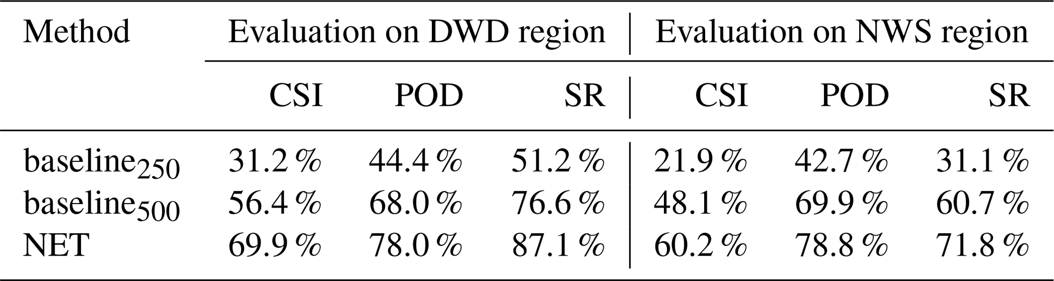
We additionally evaluated the CSI score on a coarser 0.5∘ resolution grid and compare the results against the baseline algorithm evaluated on the same grid. The used baseline does not classify its results, which is why we only display and compare the task of front detection and forgo any classification results. Due to the previously mentioned fragmentation issues, we only evaluate the results where each front may be matched against the complete set of fronts rather than just a single front object. The baseline algorithm is only designed for application in the midlatitudes and should not detect stationary fronts. Hence for this comparison we further restrict our evaluation region to fit within the midlatitudes of the Northern Hemisphere and remove stationary fronts from the labels and network output. There may be an offset between the placement of a front by the baseline and the weather services as the baseline locates its fronts at the centre of a passing front rather than the leading edge. While we believe that the used matching procedure already respects such a difference, we also evaluated the baseline method using D=500 km, i.e. doubling the search radius compared to that used in the evaluation of our network. As shown in Table 6, our network (NET) outperforms the baseline algorithm (baseline) in all evaluated scenarios and metrics with a CSI score more than twice as high when using D=250 km. Even when the baseline is evaluated with a larger search radius of D=500 km, the network outperforms it with a difference in CSI scores of more than 10 %, even though the network is still evaluated using the smaller search radius of D=250 km.
Table 6Comparison of the CSI, POD and SR of the baseline algorithm against our network for the data of 2016, restricted to the midlatitudes in the Northern Hemisphere. As the baseline algorithm does not classify fronts, we use the binary classification evaluation for our network. (Quasi-)stationary fronts were removed from the network output as well as the NWS label, because the baseline algorithm should not identify them. For the DWD label these could not be reliably removed due to the label's ambiguity. We can see that the baseline algorithm is better in predicting fronts in the DWD region than in the NWS region. Evaluation was performed at D=250 km for NET and baseline250, while D=500 km was used for baseline500. However, the network performs better in terms of all three measures for both regions.
3.1.3 Comparison of frontal climatologies
To further investigate the soundness of our front detection, we created frontal climatologies for the year 2016 for the provided weather service labels, our network and the baseline method. While the respective weather services only provide labels within their analysis region, both the network and the baseline can be executed on the entire globe. As in Sect. 3.1.2 we explicitly remove stationary fronts from both the NWS label dataset as well as the network output, when creating those climatologies. This is done as the baseline method does not include fronts propagating at less than 3 m s−1. The baseline method was designed for application within the midlatitudes, and results outside the midlatitudes should be taken with care. We therefore restrict our quantitative evaluation to regions within the midlatitudes. We nonetheless present the climatology on the global area to emphasize the difference in performance of the network compared to the baseline method outside the midlatitudes. The resulting climatologies are shown in Fig. 7.
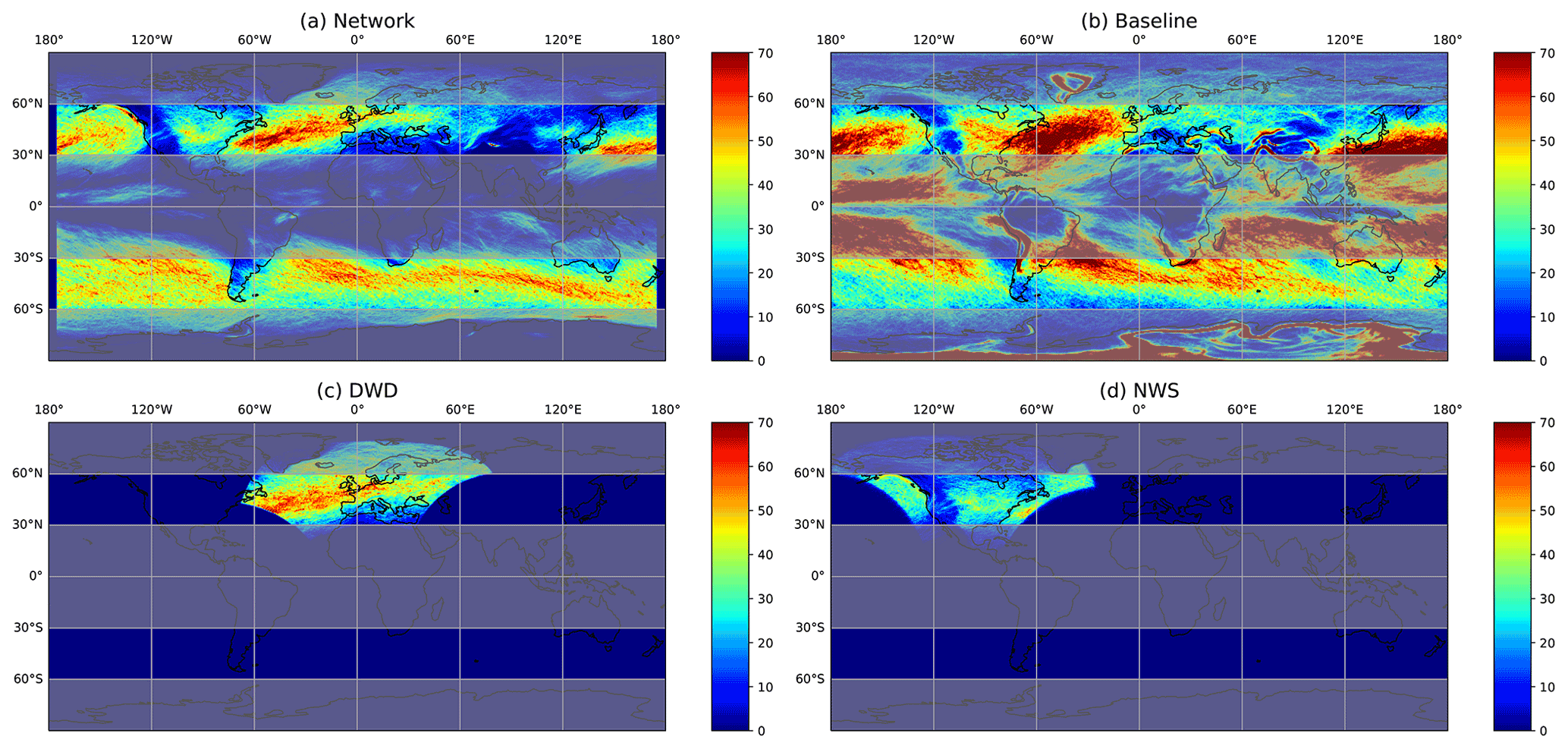
Figure 7Global frontal climatologies as derived from the ERA5 data for the year 2016 and climatologies from the weather service datasets. (a) Global frontal climatology from the network executed on the 0.25∘ grid and resampled to 0.5∘ resolution. The network does not provide a valid prediction for the outer 5∘, as the effective output domain is smaller than the input domain. For this reason no fronts are displayed here. (b) Global frontal climatology of the baseline algorithm. Note that the algorithm is not designed for application outside the midlatitudes and should only be evaluated outside the grey shaded regions. (c) Climatology of the DWD front labels. (d) Climatology of the NWS front labels. The represented front count was clipped at 70 for visual representation; regions with higher front counts are shown in red. Stationary fronts are explicitly excluded from the climatology of network-generated data and NWS-labelled data. The global climatology from the baseline algorithm does not include fronts propagating at less than 3 m s−1. The DWD dataset may include stationary fronts, as we were unable to reliably separate them from warm or cold fronts.
First, we compare the climatology for the North Atlantic–European region from the manually labelled dataset with the climatology of network-generated fronts. In the DWD climatology the North Atlantic storm track is clearly visible as a band of heightened front occurrence stretching from the East Coast of North America to the English Channel (Fig. 7c). Frontal activity tampers off inwards of the European west coast. The climatology of the network-generated fronts has a very similar overall structure with a strongly enhanced frontal frequency in the storm track region (Fig. 7a). Frontal frequency is somewhat larger at the beginning of the storm track compared to the DWD climatology. This may be related to the training with North American manual analysis, which naturally has a stronger focus on the early cyclone life cycle than the European data. Over the English Channel and North Sea coast of Europe, frontal frequency in the network-generated dataset is somewhat lower than in the DWD dataset, which may be related to the inclusion of stationary fronts in the latter but not the former. We have also seen in the previous section that very weak warm fronts, as may exist further into the European continent, are often not detected by the network. In both datasets a slightly enhanced frontal frequency around Iceland is evident.
Next, we compare the climatology for the North American region from the manually labelled dataset with the climatology of network-generated fronts. The manual labels indicate the onset of the storm track with enhanced frontal frequencies just off the North American East Coast and secondary peaks in frontal frequencies in the lee of the Rocky Mountains and along the West Coast (Fig. 7d). The climatology of network-generated fronts captures all three maxima in the frontal frequency in roughly the same location (Fig. 7a). However, frontal frequency in the lee of the Rocky Mountains and along the West Coast is more pronounced in the network-generated climatology. We are under the impression that the network tends to assign labelled warm fronts as stationary and vice versa. These shifts may explain the different frontal frequency.
Finally, we compare the global climatology of network-generated front labels to those generated by the baseline algorithm (compare Fig. 7a and b). The striking first difference between the two climatologies is the much larger spatial extent of regions with high frontal frequency in the second dataset. This is evident both in the storm track regions on both hemispheres and in the subtropical regions. In the subtropics, regions of large gradients in equivalent potential temperature exist, and these are picked up by the baseline algorithm. However, their structure and origin differ from fronts in the extratropics. It appears that the network is able to detect this difference in the structure, while focusing solely on equivalent potential temperature and frontal propagation speed is not enough information to differentiate these structures.
In absence of any manual dataset that can serve as ground truth, it is difficult to judge the physical meaningfulness of the climatological patterns emerging from either algorithm and indeed in the case of the subtropics may strongly depend on the purpose and definition of what is considered a frontal structure. In the storm track regions on both hemispheres both datasets show consistently enhanced frontal frequencies over similar geographic regions. They only differ in the zonal extent of the regions with enhanced activity and the absolute values of frontal frequencies. In the only region where we have an independent manually generated dataset often considered as the “ground truth”, the climatology of network-generated fronts is in closer agreement with the former than the climatology from the baseline algorithm. For the Southern Hemisphere or the North Pacific, we currently do not have any such dataset available.
The second striking difference is the high frontal frequency along orographic barriers in the climatology from the baseline algorithm, i.e. along the Andes, Greenland, Himalayas and Antarctic coastline. These maxima in frontal activity are largely absent from the climatology of network-generated fronts consistent with the manually labelled datasets. It appears that the network correctly discriminates between temperature and humidity gradients arising only because of the presence of significant topography and those caused by dynamically generated air mass boundaries. In contrast, focusing solely on the advection speeds in regions of large equivalent potential temperature gradients seems not to suffice.
Overall, the global picture emerging from the extrapolation of the network trained on the North American, North Atlantic and European domain also performs well on a global scale and correctly identifies regions of high frontal activity expected from previous investigations and the known general circulation patterns. While physically plausible, this is of course no vigorous evaluation of the performance of the extrapolation to different regions of the globe. Future work should investigate this aspect in a more quantitative manner with manually labelled datasets from other parts of the globe. However, overall the investigation of the front climatology agrees well with physically expected patterns and climatologies from manually generated frontal datasets. This lends additional physical credibility to the network-generated frontal labels.
A physically plausible global climatological pattern further suggests that the learned frontal identification can be extrapolated from the training region. We found that for this it is necessary to include data from two sufficiently different geographic regions, i.e. North America and North Atlantic–Europe, as well as to augment the dataset by also including zonally mirrored examples of the frontal cases (not shown). The latter was found to be particularly important for a good performance in the Southern Hemisphere. This is also visible in the Video supplement, where the general shape, composition and motion of fronts detected in the Southern Hemisphere appear plausible. At first the qualitatively good results on the Southern Hemisphere appear to contradict our claim in the previous section, that training on a single region is insufficient of extrapolation to other regions. However, we believe that this is due to the fact that this region is mostly covered by sea. As a result there is far less orographic influence in the southern regions. As such the simple mirroring of data from the North Atlantic may be sufficient to learn a seemingly good model for the sea-covered regions of the Southern Hemisphere. Nonetheless this is only a qualitative observation that needs to be explicitly evaluated, if appropriate data are available.
Table 7Extent of the regions used during comparison of climatologies. These regions correspond to the output regions used during training limited to .
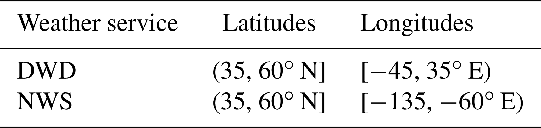
Table 8Pearson correlation coefficient of the climatology computed with the baseline algorithm (baseline) and our trained network (NET) against the climatologies created from the provided labels of the weather services for 2016. The columns denote the weather services, against which the methods were evaluated. Correlations are computed for the midlatitude regions covered by the analysis from the weather services. Stationary fronts were excluded from all climatologies except the DWD labels.
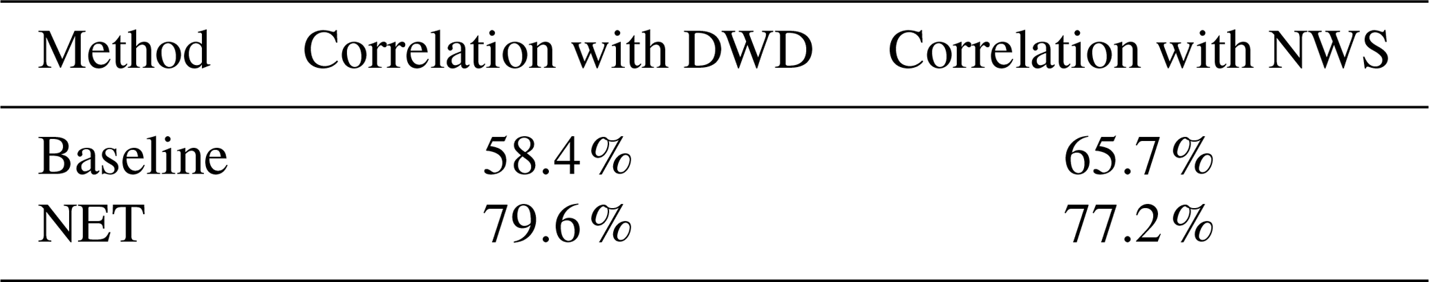
To quantify the former qualitative discussion of the climatologies, we evaluated the Pearson correlation coefficient of the created climatologies within the regions described in Table 7. The resulting correlation coefficients, provided in Table 8, show that our network outperforms the baseline algorithm in both regions with correlation coefficients greater than 77.2 %. For both regions the network results are more than 10 % higher than those of the baseline. This effect is more pronounced on the DWD dataset, which might be caused by the ambiguity of stationary fronts.
3.2 Variation in physical variables across frontal surfaces
In the previous section we showed that our proposed network can reliably detect fronts as they are provided by the weather services. In this chapter we evaluate various physical quantities across the detected frontal zone qualitatively, to assess whether or not the detected fronts express plausible physical features. Since some automatic methods such as the baseline method rely on gradients of certain thermodynamic variables, we investigate these variables for the fronts detected by our network. Thus, we can evaluate whether these fronts are detected in a completely different way or feature similar frontal characteristics as those detected by the thermodynamic methods or manual analysis.
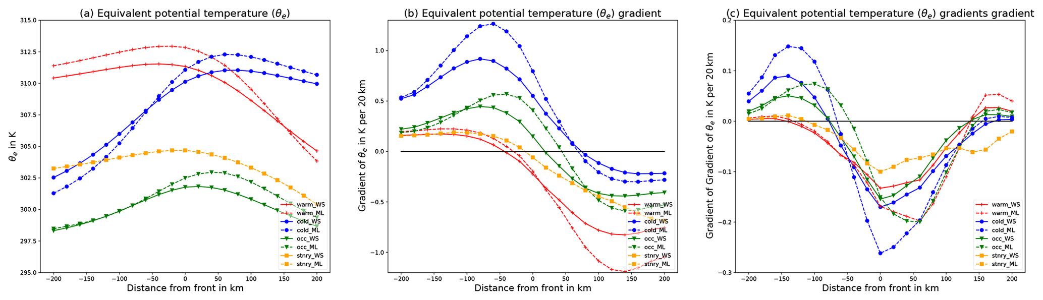
Figure 8Average value of variables at 850 hPa across fronts in the direction of wind. Mean of (a) equivalent potential temperature (θe), (b) θe gradient and (c) gradient of θe gradient with front positions determined by DWD manual analysis (solid, WS) and by our network (dashed, ML). For (b, c) we additionally display the 0 level.
For this purpose, we create cross sections perpendicular to the frontal surface for each pixel that corresponds to a front in four steps:
-
estimate the direction normal vector of the front at the given point,
-
sample points in the normal direction centred at the given point on the front,
-
calculate the mean wind direction along the sampled points,
-
use the sign of the dot product of the mean wind direction vector and the normal front vector to sort the sampled points along wind direction.
These cross sections are computed at the 850 hPa level, since the TFP methods are usually based on variables on this level. For the comparison with the thermodynamic front detection methods, we use the variable equivalent potential temperature (θe). Additionally, the variables temperature, relative humidity and (absolute) wind speed are chosen, showing important features of different front types. These variables are taken from the ERA5 dataset, while the position of the fronts is determined by our network or the weather service analyses. We used MetPy v1.0.1 to derive θe and the relative humidity (May et al., 2021). We further used GeoPy v2.2.0 (https://github.com/geopy/geopy, last access: 17 January 2022) to calculate the position of our sample points.
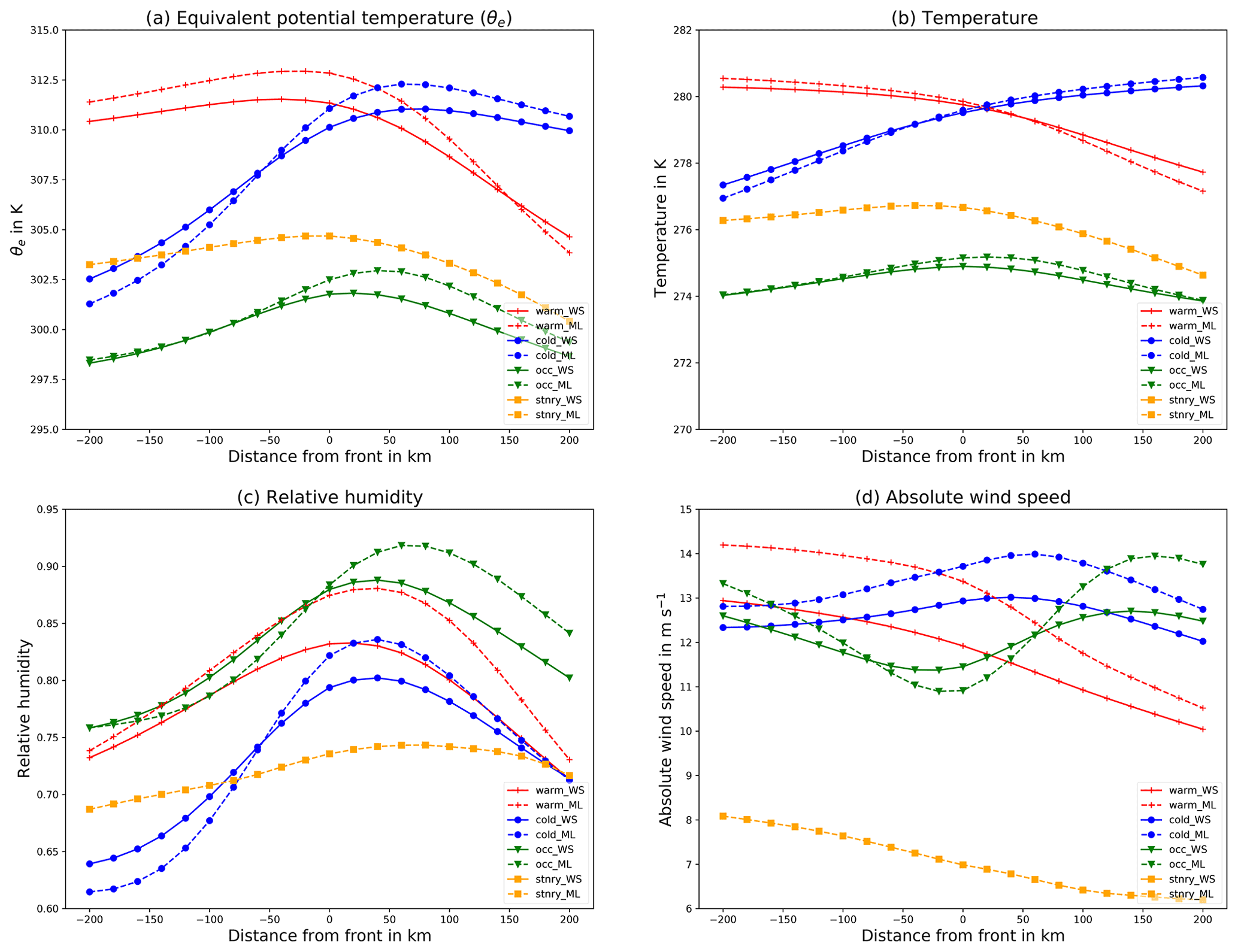
Figure 9Average value of variables at 850 hPa across the front in the direction of the wind. (a) Mean of the equivalent potential temperature (θe), (b) temperature, (c) relative humidity and (d) absolute wind speed with front positions determined by DWD manual analysis (solid, WS) and by our network (dashed, ML).
The mean cross section for the DWD frontal dataset is presented in Figs. 8 and 9. The corresponding plots for the NWS front dataset are shown in the Supplement (Figs. S2 and S3). In Fig. 8a we evaluated the variation in equivalent potential temperature (θe) at 850 hPa based on front locations (i) identified by the machine learning algorithm (dashed lines) and (ii) indicated in the surface analysis from the DWD (solid lines). For both front location datasets θe is clearly increasing (decreasing) across the frontal surface for cold (warm) fronts, as would be expected from the physical definition of these features. For the identified cold fronts the across-frontal temperature variation is on average larger than for the DWD labels. For warm fronts the across-frontal change in θe is similar for both detections, albeit the decrease ahead of the passing front is stronger for the machine learning detections. Warm fronts identified by DWD are on average located at slightly cooler temperatures. This may be explained by the assignment of some warm fronts with weak temperature gradients to the additional category of stationary fronts by our machine learning algorithm, a category non-existent in the DWD dataset. For occluded fronts there is only a small across-frontal variation in θe as could be expected, and again this is consistent across both datasets.
For most automatic front detection algorithms the across-frontal θe gradient is of importance; this quantity is shown in Fig. 8b. The θe gradient is calculated using finite differences using the sampled temperature cross sections. Again we see very similar patterns for both the DWD and our front dataset. In both datasets the frontal surface is located at the onset of a region with strong change in the horizontal θe gradient. This is consistent with the physical definition of frontal zones and agrees with the manually designed automatic front detection algorithms. Generally the network-detected fronts exhibit a stronger gradient compared to those in the weather service analysis for all types of front. Taking the gradient of the θe gradient (see Fig. 8c), we obtain a magnitude similar to the TFP, where the direction is defined by the normal of our detected front with respect to the wind direction instead of the 2D gradient of θe. For simplicity we will refer to it as approximate TFP in the following.
Several conventional methods place the front at the position where the gradient of the TFP is zero. We can clearly see this for the provided DWD labels, where all three types of front have a minimum of the approximate TFP at the frontal position. For cold fronts our networks' placement seems to agree with this. For stationary fronts the signal is less clear, but the front also appears to be located at the extremum of the approximate TFP. Differently, warm fronts and occlusions are placed with an offset of approximately 60 km to the extremum of the approximate TFP. Nonetheless we also believe that this offset is reasonable. This shows that both our used labels and the network's detections are plausible with respect to the theoretical background used for TFP methods.
As mentioned before, fronts are typically placed where the gradient of the TFP equals zero, which is thought to describe the leading edge of a front, such as it occurs with the weather service labels. The used baseline method however is different in that regard as it locates a front where the TFP equals zero, which corresponds to the centre of the frontal area. This of course creates an inherent offset in the front position. Following our evaluation as described above, we can estimate this offset is approximately 130 km (80 km) for warm (cold) fronts. Note that both distances are lower than the evaluation distances of 250 and 500 km used for the computation of performance scores in the preceding section. This highlights that the difference in CSI should not be fully accounted for by methodological difference but rather supports our statement that the network is better at the detection and placement of fronts than the baseline.
In Fig. 9 we additionally show the temperature (b), relative humidity (c) and absolute wind speed (d) across the frontal zone. The temperature variation across the frontal zone is quite similar for network- and weather-service-detected fronts and is physically reasonable. For instance, the temperature difference for warm and cold fronts is clearly visible; also, the values agree quite well. For the relative humidity, there are some differences in the absolute values; the network-detected fronts usually have enhanced relative humidity values. However, qualitatively the variation in relative humidity across the frontal zone is well captured. For warm fronts, and also occlusions, there is a pronounced maximum in RH ahead of the front, which indicates the typical frontal cloudiness. A similar signature can be seen for cold fronts, where the maximum is only slightly shifted relative to the surface front position. For the absolute wind speed, we see similar values for the different fronts (detected by network and weather services), but no pronounced structure. Note here that the mean absolute wind speed for stationary fronts is quite high (–8 m s−1) compared to the threshold criterion used by the TFP method. However, the standard deviation is also quite high (). A reason for this might be that the position of stationary fronts is not well captured by the network (also because they are only available in the NWS training dataset). Due to the uncertain position, the mean values are smeared out over a large range around the detected position. Nevertheless, the absolute wind speed at stationary fronts is much smaller than the wind speed at the others, which matches with the physical expectation that stationary fronts are moving quite slow – a feature still well captured by the network.
When comparing the frontal zone structure over North America according to NWS labels and our generated labels, generally consistent structures are also found (see Supplement), with deviations broadly mirroring those identified for the DWD data.
Overall, from the good agreement in physical structures across the identified frontal surfaces as detected by our algorithm and from the manual weather service analysis, we conclude that our algorithm detects physically meaningful positions. The positioning of the frontal surfaces is further consistent with physical intuition and interpretation prevalent in literature, and also with the physical constrains for the detection of fronts by an automatic method based on thermodynamic variables.
We can finally remark that even using the surface front as a proxy for the synoptic-scale phenomena front (as transition of air masses), the related structures for either the fronts manually determined by the weather services or automatically determined by our network are physically meaningful. This analysis shows that indeed we can use surface fronts as a ground truth for the detection of fronts in reanalysis datasets.
3.3 Correlation to extreme precipitation events
In the previous section we showed that our model detects fronts in accordance with physical expectations. We further showed that our method generally agrees with the theory of TFP methods, further demonstrating that our model predicts physically plausible fronts. In this chapter we will further validate our results and at the same time provide an example of how our proposed method may be applied in a scientific context aside from pure front detection for operational weather forecasts. To do this we evaluate how weather fronts as detected by our network are connected to extreme precipitation. We present the results (i) for the occurrence of extreme precipitation if there is already a front (Sect. 3.3.2), and (ii) for the presence of a front if an extreme event occurs at a grid point (Sect. 3.3.4).
3.3.1 Data and terminology
Catto and Pfahl (2013) previously investigated the co-occurrence of fronts and extreme precipitation using a front detection algorithm based on thermal front parameters (TFP) and the ERA-Interim dataset. Due to the used front detection algorithm, they evaluated their results on a 2.5∘ spatial resolution, and they only use the 6-hourly accumulated precipitation variable of ERA-Interim.
Differently to Catto and Pfahl (2013), our front detection can be applied to the 0.25∘ resolution of the ERA5 dataset to provide a more detailed evaluation. Additionally, ERA5 provides data at an hourly interval, allowing us to evaluate at a 6 times higher temporal resolution. Unlike Catto and Pfahl (2013), we decided to use the 1-hourly accumulated total precipitation to match the temporal resolution of our data samples. As all evaluation data are taken directly from the ERA5 grid, we do not need to perform any resampling of data. We evaluate the data for a near-global region spanning from and . Grid points poleward of 60∘ are excluded as in Catto and Pfahl (2013), while the restriction in the longitudinal direction is caused by our network's reduced output domain size. We further mask regions with high topography (>2000 m) from the evaluation. This filtering mostly removes stationary fronts associated with mountainous terrain.
Extreme precipitation is defined as any precipitation exceeding the 99th percentile of precipitation at a given grid point over the considered 9-year period (2010–2018). The correlation of fronts with extreme precipitation events and vice versa is investigated for the year 2016 only. We consider a grid point to be associated with any event (e.g. a front or extreme precipitation) if such an event occurs within a predefined attribution radius. If not explicitly stated otherwise, the attribution radius is chosen similar to Catto and Pfahl (2013) to be 2.5∘, albeit our attribution radius is a bit more accurate, due to the higher resolution of the ERA5 grid. To decide whether a connection between extreme precipitation and fronts is significant, we conduct a statistical test using statsmodels v0.12.2 (Seabold and Perktold, 2010) for the quantile regression. For our investigations, we adopted the test procedure as described in the study by Pfahl and Wernli (2012). A more detailed description of the methodology of this section can be found in Sect. S5.
3.3.2 Extreme precipitation associated with fronts
In Tables 9 and 10 the proportion of extreme precipitation events at grid points that can be associated with a front (R1) is presented for different regions. For comparison with the former work by Catto and Pfahl (2013), we report values for the global evaluation, i.e. including the tropics, although the application of front detection methods in these regions remains questionable. In addition, we present a more detailed analysis for different parts of the midlatitudes (Table 10). We can clearly observe that a high proportion of extreme precipitation events can be associated with fronts when considering sea-covered regions. Filtering out mountainous regions, the correlation between extreme precipitation and fronts increases compared to the full midlatitude dataset. Over flat terrain, the frontal systems can develop in a quasi idealized fashion; thus warm, cold and occlusion fronts can develop quite undisturbed. Thus, extreme precipitation is mostly linked to the large-scale features, whereas over (steep) terrain local effects can disturb the frontal development and/or generate extreme precipitation by other processes. This effect also explains why R1 is higher for the southern midlatitudes or hemisphere compared to their northern counterparts. Further we can see that R1 is higher for the midlatitudes than for the tropics for all types except stationary fronts, where we observe the opposite effect. This is expected as it coincides with the frontal frequency at these locations and the presence of other processes generating extreme precipitation, e.g. organized deep convection. While stationary fronts are more often detected near high-altitude regions, above land surface and at the Intertropical Convergence Zone (ITCZ), the other types of fronts tend to occur more often over the ocean, e.g. the storm tracks in the Atlantic and Pacific. This is in accordance with the correlations shown in Tables 9 and 10, where we can see the same connections for R1.
Table 9Average proportion of extreme precipitation events associated with a front for different regions in 2016. Results are shown separately for the entire globe ( N), Northern Hemisphere and Southern Hemisphere ( N and S respectively), and tropics ( N).
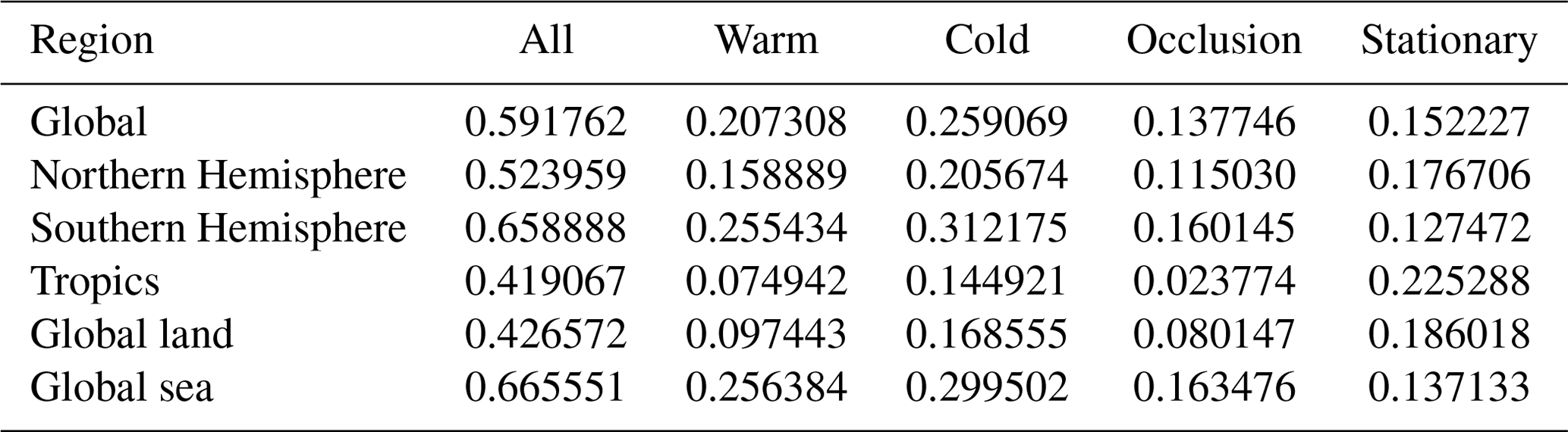
Table 10Average proportion of extreme precipitation events associated with a front for different regions in 2016 for the midlatitudes ( N and S respectively).
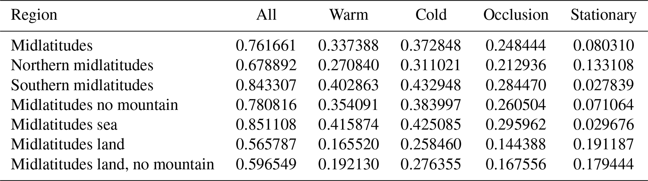
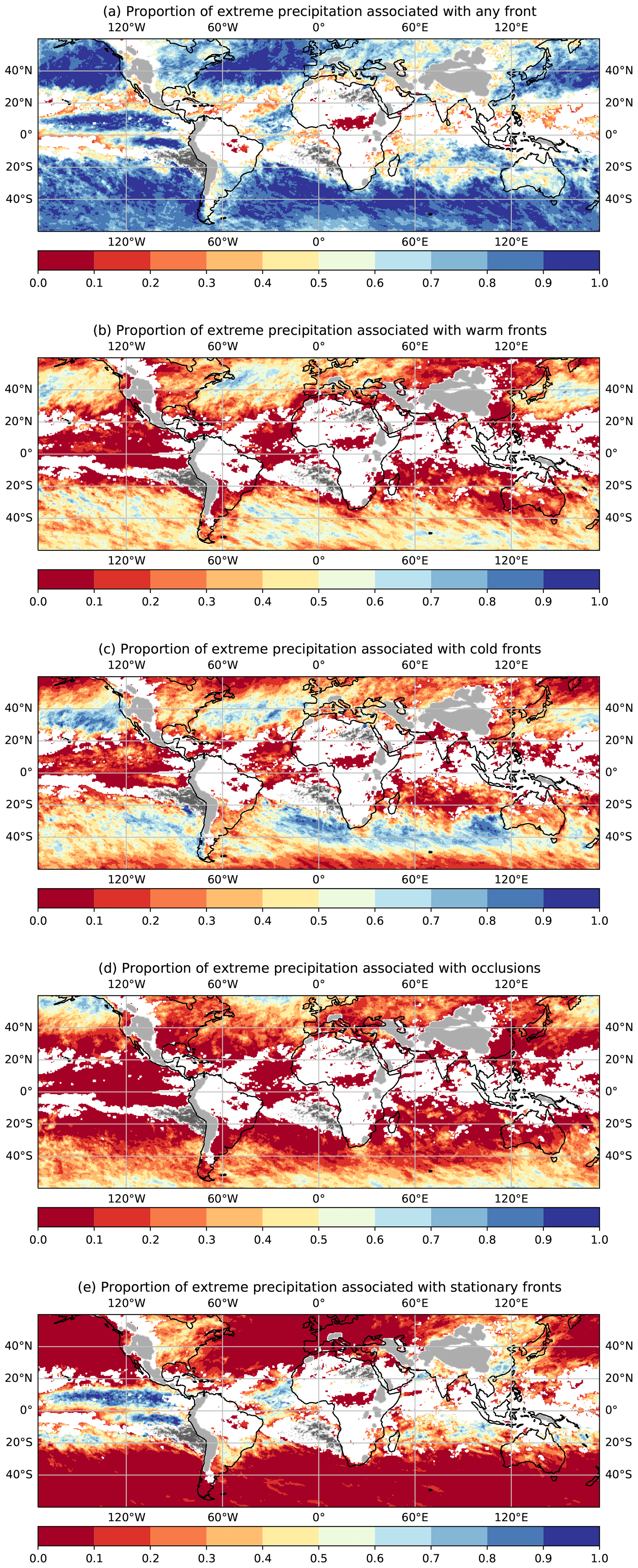
Figure 10Proportion of extreme precipitation events, which are associated with a front. Regions with high topography are shaded in light grey, while areas where no extreme precipitation events occurred in 2016 are shaded in dark grey. Regions where no significant correlation between extreme precipitation and fronts was found are blank. Results are shown for (a) any front, (b) warm fronts, (c) cold fronts, (d) occlusions and (e) stationary fronts.
Figure 10 displays R1 for each frontal type at each grid cell. For this plot all high-altitude regions are shaded grey (light grey), while all regions where no significant connections between fronts and extreme precipitation could be found are shaded white. Further, we masked all regions where no extreme precipitation event was found using a dark grey overlay. This occurs since extreme precipitation is defined using all years from 2010 to 2018, while correlations to fronts are only investigated for the year 2016. In some storm track regions over the ocean, more than 90 % of all extreme precipitation events can be associated with a front. Overall extreme precipitation appears to be more often associated with cold fronts than warm fronts. In the northern midlatitudes we can see that extreme precipitation events associated with warm fronts occur farther north than those associated with cold fronts. For occlusions this is even clearer as the highest proportion of extreme precipitation associated with occlusions is found close to 60∘ N. For the Southern Hemisphere, a similar tendency can be seen, even though the local maxima in the correlation are not as clearly visible. As previously mentioned, stationary fronts are less often found over midlatitude oceanic regions, and therefore unsurprisingly almost no extreme precipitation events are associated with stationary fronts there. In contrast, extreme precipitation events in the tropics, especially at the ITCZ, are more likely to be associated with stationary fronts. Similarly the eastern parts of North America and land surfaces near the northeastern Pacific coast of Asia also have a relatively high percentage of extreme precipitation events associated with stationary fronts.
Note that for the tropics the detection of fronts is quite questionable. However, for comparison with Catto and Pfahl (2013) using a TFP front detection method, these regions are included, although front detection methods are generally designed for and therefore applicable in a meaningful way only for the extratropics. Overall our results are in good agreement with those derived in Catto and Pfahl (2013).
3.3.3 Extreme precipitation associated with fronts relative to frontal frequency
In Fig. 11 we display R1 as a function of the frequency of a point being associated with a front (Pa(fr)) at all. Additionally we plotted the 1st and 99th percentiles derived from the statistical test (for details see Sect. S5.2) as well as the identity as orientation. The lines and box plots can be interpreted as follows: if the box plot is above the 99th percentile line, we can conclude that the correlation between extreme precipitation events and fronts is significant in terms of our statistical test.
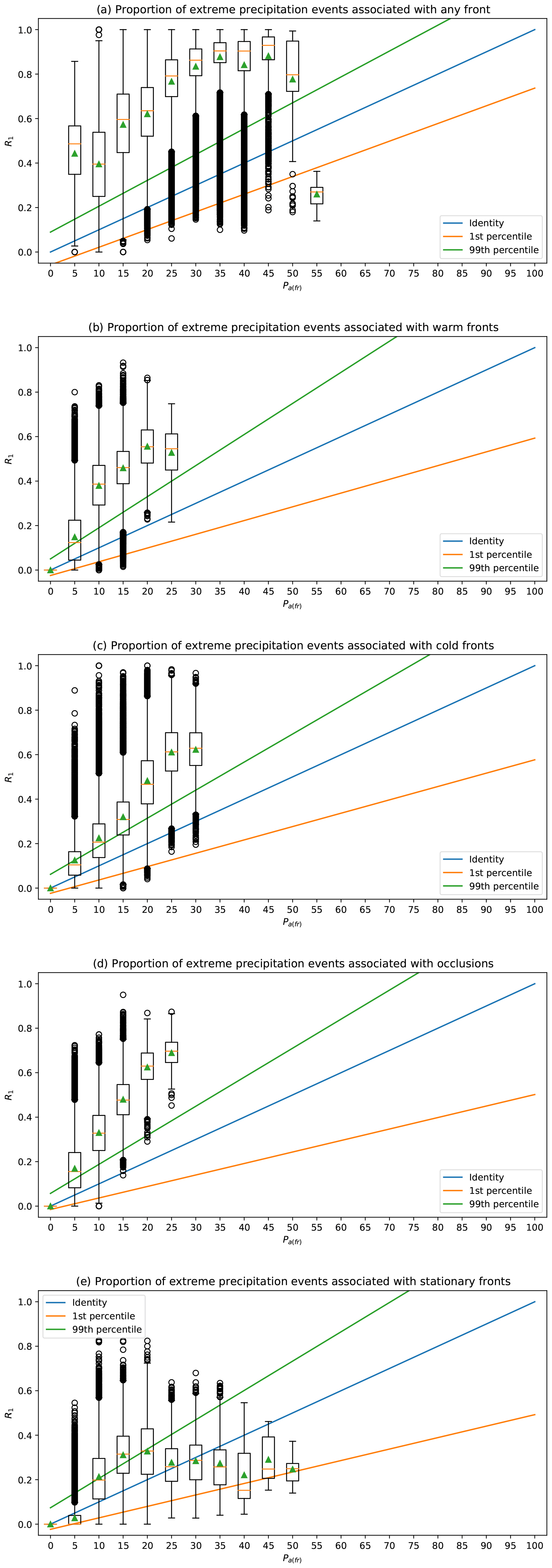
Figure 11Fraction of extreme precipitation events grouped by frontal frequency as boxplots. Including 1st and 99th percentiles of the statistical test. Results are shown for (a) any front, (b) warm fronts, (c) cold fronts, (d) occlusions and (e) stationary fronts.
For warm fronts, cold fronts and occlusions, we find that both the median and the mean of each bin exceed the 99th percentile even for small front frequencies; i.e. a significant correlation between fronts and extreme precipitation exists. For stationary fronts this appears less clear: up to 20 % frontal frequency the curve connecting the medians indicates a significant correlation between extreme precipitation and stationary fronts, before flattening towards points with larger frontal frequencies. Considering all types of fronts together (Fig. 11a), the mean and median R1 exceed the 99th percentile for all frontal frequency bins except the largest Pa(fr) bin. This clearly indicates a strong connection between fronts and extreme precipitation.
3.3.4 Fronts associated with extreme precipitation
In the previous section we have shown that a high percentage of extreme precipitation events are associated with a front. We also found that outside the tropics this connection is statistically significant according to the performed test (details found in S5). However, we are also interested in the proportion of fronts that are associated with extreme precipitation events (R2). Similar to Fig. 10 we plotted R2 per grid point in Fig. 12. Light grey and white shaded regions are masked as before, while regions where no front of the corresponding type occurred are shaded in dark grey. In general, over large swaths of the midlatitudes more than 40 % of fronts are associated with extreme precipitation. Also, regions where a front is less likely to occur tend to have a higher percentage of fronts associated with extreme precipitation. This is very clear for the occlusions: according to the climatology presented, earlier occlusions are predominantly found in the more poleward midlatitude region, but occlusions occurring close to 30∘ N/S are almost always associated with extreme precipitation. The decrease in R2 for regions with a higher relative frontal frequency (Pfr) can at least partially be explained by the definition of extreme precipitation events, as it inherently limits the number of such events. If Pfr exceeds that amount, it is likely that several fronts may not be associated with an extreme precipitation event, even though strong precipitation still occurs. This is somewhat dampened by the fact that for R2 a grid point with a front only needs to be within the attribution radius of an extreme precipitation event to give each front several grid points to be associated with. Compared to Catto and Pfahl (2013), our results show the same tendencies, but in our analysis a larger fraction of fronts are associated with extreme precipitation events than in their work.
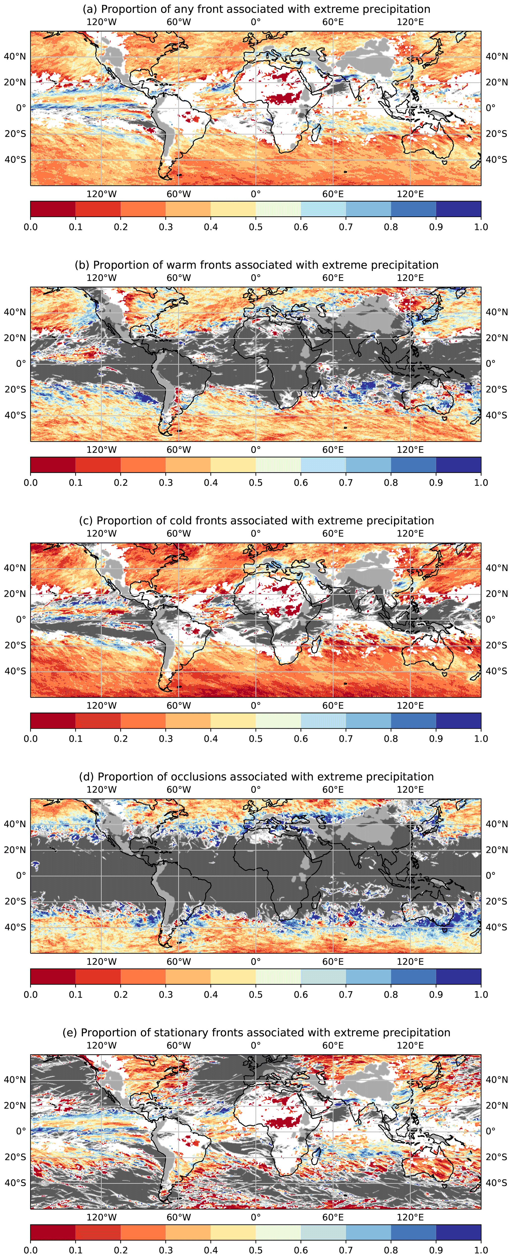
Figure 12Proportion of fronts that are associated with an extreme precipitation event. Regions with high topography are shaded in light grey, while areas where no fronts of the corresponding class were detected in 2016 are shaded in dark grey. Regions where no significant correlation between extreme precipitation and fronts was found are blank. Results are shown for (a) any front, (b) warm fronts, (c) cold fronts, (d) occlusions and (e) stationary fronts.
Overall our results show a significant connection between extreme precipitation and fronts detected by our network. Our results generally agree with the results of the previous study by Catto and Pfahl (2013). We additionally investigated the correlation between fronts and extreme precipitation at a higher resolution, i.e. for two smaller attribution radii of 5 px (1.25∘) and 2 px (0.5∘). The qualitative features (i.e. the regions with high correlations) remain the same, but the correlation magnitude is reduced due to the smaller radius of influence. The respective figures can be found in Fig. S4. This once again highlights the potential of our network to be used in future scientific research. Such investigations cannot be carried out with classical TFP methods, since they are on a global scale (i.e. using fixed thresholds) most likely restricted to low-resolution datasets. This underlines the benefit of our new method over existing ones.
Atmospheric fronts are important features that are usually associated with synoptic-scale weather systems. Since fronts are usually connected with significant weather, e.g. clouds and precipitation, and occasionally with extreme precipitation events, they are of high interest for weather forecasts but also in terms of scientific research of such events. While the term front refers to a sharp transition between air masses of different characteristics (e.g. in terms of temperature and humidity), there is unfortunately not a generally accepted definition of a front. This is also reflected in many different approaches to detect fronts automatically, e.g. using (multiple) gradients of thermodynamic variables, or even recently using machine learning techniques.
In this study we present a new method for automatic front detection based on a neural network, which uses ERA5 reanalysis data. As a ground truth for training and validation, we use surface front data from two different weather services (NWS and DWD) covering significant parts of the Northern Hemisphere; for validation a disjoint subset of this dataset is used. We train the network on a loss function that allows to classify and predict fronts across the input regions. Our applied loss function results in the network predicting clearly localized fronts without the need of morphological post-processing thinning operations. The network is able to predict fronts with a critical success rate higher than about 66.9 % and an object detection rate higher than about 77 %.
For a better evaluation of the quality of the method, we compare the network output with a baseline method, which uses a traditional approach operating on thermodynamic variables (TFP approach). For both methods a climatology of fronts is derived. In this direct comparison, the new method outperforms the baseline method in the direct comparison with the data from the weather services. We can show that we cannot simply transfer a locally trained network onto any other region but rather need to train on several datasets to obtain a reliable general front detection. The climatology results indicate that a transfer to oceanic regions may be feasible; however this has to be evaluated in future research. It is also desirable to further investigate up to which degree extrapolation onto different regions is possible and to investigate whether or not generalization onto global data is possible from just a few subregions.
The evaluation of physical properties relative to the network-detected fronts shows that our detected fronts generally exhibit similar properties as those usually looked for in classical methods. As an example gradients in the equivalent potential temperature are shown. In addition, a similar quantity as for classical TFP methods is determined from equivalent potential temperature. In the comparison of these quantities relative to fronts determined by the weather services and detected by the network, we find very good agreement; in addition, they exhibit the same features as would be detected by a TFP method. This also shows that our ground truth data, surface fronts originating from two weather services, are a suitable choice; although surface fronts are detected, they show the correct structure in terms of thermodynamic variables. Thus, surface fronts can serve as a proxy for the detection of fronts; however our analysis shows that the resulting fronts are meaningful.
In a final application, we investigate the connection of fronts with extreme precipitation events. This investigation is guided by the former investigation by Catto and Pfahl (2013); however, our network allows us to fully use the available resolution of ERA5 and to investigate characteristics of fronts at a high spatial and temporal resolution, leading to a more detailed investigation. For the midlatitudes the connection between extreme precipitation events and front occurrence is found to be most prominent, with the strongest correlation over flat terrain, especially over the ocean. This application shows that our new front detection method is not only just a tool for operational weather forecasting but also useful for scientific investigations. Since the method can be applied to high-resolution data, this is a clear benefit of the new method over existing TFP methods, which are usually restricted to low-resolution datasets or heavily rely on smoothing operators. In addition, the method is quite flexible, and it is quite straightforward to include new training datasets, such as surface fronts for the Southern Hemisphere. In addition, there is no principle obstacle for using meteorological datasets with higher resolution as input for the method.
In future work separating the detection from the classification task may be beneficial, seeing the good detection rates of the presented network in the binary case. We would also like to further explore the application and effect of other methods to handle the label bias, such as the method described by Acuna et al. (2019). In terms of research in the field of meteorology, we want to apply this method for further research on the connection of frontal systems with other phenomena, e.g. for the investigation of clouds at different heights around fronts or transport phenomena associated with frontal systems.
The latest code is available at https://doi.org/10.5281/zenodo.5783934 (Niebler, 2021b). ERA5 reanalysis data can be accessed via the ECMWF climate data centre. The used NWS frontal label is available at https://doi.org/10.5281/zenodo.2642801 (National Weather Service, 2019). Our extracted polylines of the DWD data are available at https://doi.org/10.5281/zenodo.5785816 (Niebler, 2021a).
A video supplement showing predicted fronts for January 2016 is available at https://doi.org/10.5446/54716 (Niebler, 2021c).
The supplement related to this article is available online at: https://doi.org/10.5194/wcd-3-113-2022-supplement.
SN implemented and trained the network. He also evaluated the baseline method as well as the network. BS, AM, PS, and SN wrote the draft of the paper. BS, AM, and PS proposed and supervised the project. All authors edited the paper and analysed the results.
The contact author has declared that neither they nor their co-authors have any competing interests.
Publisher's note: Copernicus Publications remains neutral with regard to jurisdictional claims in published maps and institutional affiliations.
The study is supported by the project “Big Data in Atmospheric Physics (BINARY)”, funded by the Carl Zeiss Foundation (grant P2018-02-003). We acknowledge the ECMWF for providing access to the ERA5 reanalysis data. We further acknowledge ETH Zurich and especially Michael Sprenger for providing the code for the used baseline method. Label data for the European continent and North Atlantic were provided by the Deutscher Wetterdienst. Label data for the North American continent were provided and made publicly available by the North American Weather Service. We further acknowledge the ZDV of the Johannes Gutenberg University and the Mogon II Super Cluster for providing the necessary hardware and computing time to execute our experiments. We thank Philipp Reutter, Michael Wand and Holger Tost for fruitful discussions.
This research has been funded by the Carl-Zeiss-Stiftung (grant no. P2018-02-003).
This paper was edited by Lukas Papritz and reviewed by two anonymous referees.
Acuna, D., Kar, A., and Fidler, S.: Devil is in the Edges: Learning Semantic Boundaries from Noisy Annotations, in: Proceedings of the IEEE/CVF Conference on Computer Vision and Pattern Recognition, 11075–11083, 2019. a
Berry, G., Reeder, M. J., and Jakob, C.: A global climatology of atmospheric fronts, Geophys. Res. Lett., 38, L04809, https://doi.org/10.1029/2010GL046451, 2011. a, b
Biard, J. C. and Kunkel, K. E.: Automated detection of weather fronts using a deep learning neural network, Adv. Stat. Clim. Meteorol. Oceanogr., 5, 147–160, https://doi.org/10.5194/ascmo-5-147-2019, 2019. a, b, c, d, e
Bitsa, E., Flocas, H., Kouroutzoglou, J., Hatzaki, M., Rudeva, I., and Simmonds, I.: Development of a Front Identification Scheme for Compiling a Cold Front Climatology of the Mediterranean, Climate, 7, 130, https://doi.org/10.3390/cli7110130, 2019. a
Bochenek, B., Ustrnul, Z., Wypych, A., and Kubacka, D.: Machine Learning-Based Front Detection in Central Europe, Atmosphere, 12, 1312, https://doi.org/10.3390/atmos12101312, 2021. a
Brooks, H. E.: Tornado-Warning Performance in the Past and Future: A Perspective from Signal Detection Theory, B. Am. Meteorol. Soc., 85, 837–844, https://doi.org/10.1175/BAMS-85-6-837, 2004. a
Catto, J. and Dowdy, A.: Understanding compound hazards from a weather system perspective, Weather and Climate Extremes, 32, 100 313, https://doi.org/10.1016/j.wace.2021.100313, 2021. a
Catto, J., Madonna, E., Joos, H., Rudeva, I., and Simmonds, I.: Global Relationship between Fronts and Warm Conveyor Belts and the Impact on Extreme Precipitation, J. Climate, 28, 8411–8429, https://doi.org/10.1175/JCLI-D-15-0171.1, 2015. a
Catto, J. L. and Pfahl, S.: The importance of fronts for extreme precipitation, J. Geophys. Res.-Atmos., 118, 10791–10801, https://doi.org/10.1002/jgrd.50852, 2013. a, b, c, d, e, f, g, h, i, j, k
DWD – Deutscher Wetterdienst: Deutscher Wetterdienst Webpage, available at: https://www.dwd.de/, last access: 15 December 2021. a, b
ECMWF: L137 model level definitions, available at: https://www.ecmwf.int/en/forecasts/documentation-and-support/137-model-levels, last access: 18 May 2021. a
Foss, M., Chou, S. C., and Seluchi, M. E.: Interaction of cold fronts with the Brazilian Plateau: a climatological analysis, Int. J. Climatol., 37, 3644–3659, https://doi.org/10.1002/joc.4945, 2017. a
Hersbach, H., Bell, B., Berrisford, P., Hirahara, S., Horányi, A., Muñoz-Sabater, J., Nicolas, J., Peubey, C., Radu, R., Schepers, D., Simmons, A., Soci, C., Abdalla, S., Abellan, X., Balsamo, G., Bechtold, P., Biavati, G., Bidlot, J., Bonavita, M., De Chiara, G., Dahlgren, P., Dee, D., Diamantakis, M., Dragani, R., Flemming, J., Forbes, R., Fuentes, M., Geer, A., Haimberger, L., Healy, S., Hogan, R. J., Hólm, E., Janisková, M., Keeley, S., Laloyaux, P., Lopez, P., Lupu, C., Radnoti, G., de Rosnay, P., Rozum, I., Vamborg, F., Villaume, S., and Thépaut, J.-N.: The ERA5 global reanalysis, Q. J. Roy. Meteor. Soc., 146, 1999–2049, https://doi.org/10.1002/qj.3803, 2020. a, b
Hewson, T. D.: Objective fronts, Meteorol. Appl., 5, 37–65, https://doi.org/10.1017/S1350482798000553, 1998. a, b
Hewson, T. D. and Titley, H. A.: Objective identification, typing and tracking of the complete life-cycles of cyclonic features at high spatial resolution, Meteorol. Appl., 17, 355–381, https://doi.org/10.1002/met.204, 2010. a
Hope, P., Keay, K., Pook, M., Catto, J., Simmonds, I., Mills, G., McIntosh, P., Risbey, J., and Berry, G.: A Comparison of Automated Methods of Front Recognition for Climate Studies: A Case Study in Southwest Western Australia, Mon. Weather Rev., 142, 343–363, https://doi.org/10.1175/MWR-D-12-00252.1, 2014. a
Hu, Y., Deng, Y., Lin, Y., Zhou, Z., Cui, C., and Dong, X.: Dynamics of the spatiotemporal morphology of Mei-yu fronts: an initial survey, Clim. Dynam., 56, 2715–2728, https://doi.org/10.1007/s00382-020-05619-2, 2021. a
Jakob, W., Rhinelander, J., and Moldovan, D.: pybind11 – Seamless operability between C++11 and Python, GitHub [code], https://github.com/pybind/pybind11 (last access: 17 January 2022), 2017. a
Jenkner, J., Sprenger, M., Schwenk, I., Schwierz, C., Dierer, S., and Leuenberger, D.: Detection and climatology of fronts in a high-resolution model reanalysis over the Alps, Meteorol. Appl., 17, 1–18, https://doi.org/10.1002/met.142, 2010. a, b, c, d
Lagerquist, R., McGovern, A., and II, D. J. G.: Deep Learning for Spatially Explicit Prediction of Synoptic-Scale Fronts, Weather Forecast., 34, 1137–1160, https://doi.org/10.1175/WAF-D-18-0183.1, 2019. a, b, c, d, e, f, g, h, i
Martius, O., Pfahl, S., and Chavalier, C.: A global quantification of compound precipitation and wind extremes, Geophys. Res. Lett., 43, 7709–7717, https://doi.org/10.1002/2016GL070017, 2016. a
Matsuoka, D., Sugimoto, S., Nakagawa, Y., Kawahara, S., Araki, F., Onoue, Y., Iiyama, M., and Koyamada, K.: Automatic Detection of Stationary Fronts around Japan Using a Deep Convolutional Neural Network, SOLA, 15, 154–159, https://doi.org/10.2151/sola.2019-028, 2019. a, b, c, d
May, R. M., Arms, S. C., Marsh, P., Bruning, E., Leeman, J. R., Goebbert, K., Thielen, J. E., Bruick, Z. S., and Camron, M. D.: MetPy: A Python Package for Meteorological Data, UCAR [code], https://doi.org/10.5065/D6WW7G29, 2021. a
Mesinger, F., DiMego, G., Kalnay, E., Mitchell, K., Shafran, P. C., Ebisuzaki, W., Jović, D., Woollen, J., Rogers, E., Berbery, E. H., Ek, M. B., Fan, Y., Grumbine, R., Higgins, W., Li, H., Lin, Y., Manikin, G., Parrish, D., and Shi, W.: North American Regional Reanalysis, B. Am. Meteorol. Soc., 87, 343–360, https://doi.org/10.1175/BAMS-87-3-343, 2006. a
National Weather Service: National Weather Service Coded Surface Bulletins, 2003-, Zenodo [data set], https://doi.org/10.5281/zenodo.2642801, 2019. a, b
Niebler, S.: Front polylines extracted from DWD Maps, Zenodo [data set], https://doi.org/10.5281/zenodo.5785816, 2021a. a
Niebler, S.: FrontDetection, Zenodo [code], https://doi.org/10.5281/zenodo.5783934, 2021b. a
Niebler, S.: Detected Fronts January 2016, TIB-AV Portal, https://doi.org/10.5446/54716, 2021c. a, b, c
Parfitt, R., Czaja, A., and Seo, H.: A simple diagnostic for the detection of atmospheric fronts, Geophys. Res. Lett., 44, 4351–4358, https://doi.org/10.1002/2017GL073662, 2017. a
Paszke, A., Gross, S., Massa, F., Lerer, A., Bradbury, J., Chanan, G., Killeen, T., Lin, Z., Gimelshein, N., Antiga, L., Desmaison, A., Kopf, A., Yang, E., DeVito, Z., Raison, M., Tejani, A., Chilamkurthy, S., Steiner, B., Fang, L., Bai, J., and Chintala, S.: PyTorch: An Imperative Style, High-Performance Deep Learning Library, in: Advances in Neural Information Processing Systems 32, edited by Wallach, H., Larochelle, H., Beygelzimer, A., d'Alché-Buc, F., Fox, E., and Garnett, R., 8024–8035, Curran Associates, Inc. [code], http://papers.neurips.cc/paper/9015-pytorch-an-imperative-style-high-performance-deep-learning-library.pdf (last access: 17 January 2022), 2019. a
Pfahl, S. and Wernli, H.: Quantifying the Relevance of Cyclones for Precipitation Extremes, J. Climate, 25, 6770–6780, https://doi.org/10.1175/JCLI-D-11-00705.1, 2012. a
Renard, R. J. and Clarke, L. C.: Experiments In Numerical Objective Frontal Analysis, Mon. Weather Rev., 93, 541–556, 1965. a
Ribeiro, B. Z., Seluchi, M. E., and Chou, S. C.: Synoptic climatology of warm fronts in Southeastern South America, Int. J. Climatol., 36, 644–655, https://doi.org/10.1002/joc.4373, 2016. a
Ronneberger, O., Fischer, P., and Brox, T.: U-Net: Convolutional Networks for Biomedical Image Segmentation, in: International Conference on Medical image computing and computer-assisted intervention, Springer, 234–241, 2015. a, b
Sanders, F.: A proposed method of surface map analysis, Mon. Weather Rev., 127, 945–955, https://doi.org/10.1175/1520-0493(1999)127<0945:APMOSM>2.0.CO;2, 1999. a
Schemm, S., Rudeva, I., and Simmonds, I.: Extratropical fronts in the lower troposphere – global perspectives obtained from two automated methods, Q. J. Roy. Meteor. Soc., 141, 1686–1698, https://doi.org/10.1002/qj.2471, 2015. a, b, c, d, e, f
Schemm, S., Sprenger, M., and Wernli, H.: When During Their Life Cycle Are Extratropical Cyclones Attended By Fronts?, B. Am. Meteorol. Soc., 99, 149–166, https://doi.org/10.1175/BAMS-D-16-0261.1, 2018. a, b
Schulzweida, U.: CDO User Guide, Zenodo [code], https://doi.org/10.5281/zenodo.3539275, 2019. a
Seabold, S. and Perktold, J.: statsmodels: Econometric and statistical modeling with python, in: 9th Python in Science Conference, Austin, TX, 61 pp., 2010. a
Shakina, N. P.: Identification of zones of atmospheric fronts as a problem of postprocessing the results of numerical prediction, Russ. Meteorol. Hydro+, 39, 1–10, https://doi.org/10.3103/S1068373914010014, 2014. a, b
Shelhamer, E., Long, J., and Darrell, T.: Fully Convolutional Networks for Semantic Segmentation, IEEE T. Pattern Anal., 39, 640–651, https://doi.org/10.1109/TPAMI.2016.2572683, 2017. a
Simmonds, I., Keay, K., and Bye, J. A. T.: Identification and Climatology of Southern Hemisphere Mobile Fronts in a Modern Reanalysis, J. Climate, 25, 1945–1962, https://doi.org/10.1175/JCLI-D-11-00100.1, 2012. a
Thomas, C. M. and Schultz, D. M.: Global Climatologies of Fronts, Airmass Boundaries, and Airstream Boundaries: Why the Definition of “Front” Matters, Mon. Weather Rev., 147, 691–717, https://doi.org/10.1175/MWR-D-18-0289.1, 2019a. a
Thomas, C. M. and Schultz, D. M.: What are the Best Thermodynamic Quantity and Function to Define a Front in Gridded Model Output?, B. Am. Meteorol. Soc., 100, 873–896, https://doi.org/10.1175/BAMS-D-18-0137.1, 2019b. a
Uccellini, L., Corfidi, S., Junker, N., Kocin, P., and Olson, D.: Report On The Surface-Analysis Workshop Held At The National-Meteorological-Center – 25–28 March 1991, B. Am. Meteorol. Soc., 73, 459–472, 1992. a
A tuning of the method for the 0.25∘ resolution was not possible, since features on small scales disturb the evaluation of the gradients.